IQ Plot- Python
The purpose of this tutorial is to show how to plot IQ data that are captured from sdr_spectrum or Remote API. There are multiple ways to capture IQ data that can be processed by the example in this tutorial. Refer to following tutorials regarding the way to capture IQ data.
Table of Contents
Introduction
In radio frequency (RF) and signal processing domains, IQ data (In-phase and Quadrature data) represents the complex-valued samples acquired from software-defined radios (SDRs) or similar digitizing hardware. This data is fundamental for analyzing, demodulating, and visualizing signals across a wide range of wireless communication and spectrum monitoring applications. Technologies such as sdr_spectrum and Remote API frameworks enable users to capture raw IQ samples directly from radio front-ends, storing them in standard formats for offline or real-time analysis. Plotting IQ data is a critical step in understanding signal characteristics such as bandwidth, modulation scheme, and interference patterns. This tutorial focuses on demonstrating how to efficiently plot IQ data that has been acquired via sdr_spectrum or Remote API, using Python as the primary data processing and visualization tool. The provided Python script illustrates advanced data handling, offering flexible options for users to process and visualize IQ files, whether for quick inspection or in-depth analysis. By leveraging Python’s mature scientific libraries, users can gain actionable insights into their captured RF environments, making this process an essential skill for engineers, researchers, and hobbyists working with SDR platforms and RF analytics.
-
Context of the Technology
- IQ data forms the backbone of all digital signal processing in SDR systems, encapsulating amplitude and phase information that allows for complete signal reconstruction and analysis.
- sdr_spectrum and Remote API are widely adopted tools for capturing IQ data, supporting a variety of SDR hardware and remote operation scenarios.
- Python, with libraries like NumPy and Matplotlib, offers a powerful ecosystem for scientific computing, making it ideal for processing and visualizing complex IQ data.
-
Relevance and Importance of This Tutorial
- Understanding how to plot and interpret IQ data is crucial for RF engineers, SDR developers, and researchers working in wireless communications, spectrum monitoring, and interference detection.
- This tutorial provides a mature, feature-rich example Python script for processing IQ data, offering capabilities beyond basic plotting, such as data selection and post-processing.
- Users can adapt the script for their own RF analysis workflows, increasing productivity and deepening their understanding of SDR-acquired signals.
-
Learning Outcomes
- Gain practical experience in handling and visualizing IQ data files using Python.
- Learn how to leverage advanced options in the provided script for flexible data processing.
- Develop the ability to interpret visual representations of RF signals for further analysis or development tasks.
-
Prerequisite Knowledge and Skills
- Basic understanding of RF concepts and signal processing terminology, including the meaning of IQ data.
- Familiarity with Python programming and core scientific libraries (NumPy, Matplotlib).
- Access to IQ data files acquired via sdr_spectrum or Remote API as referenced in related tutorials.
- For users seeking minimalistic examples, a simpler tutorial is available and should be consulted for basic IQ file format understanding.
-
Scope and Support
- This tutorial provides a comprehensive example script for plotting IQ data, but does not cover Python technical support or detailed IQ data acquisition methods (refer to linked tutorials for those).
- The focus is on demonstrating practical usage and extensibility of the script for advanced RF data visualization.
Summary of the Tutorial
This tutorial provides detailed procedures for testing and visualizing IQ (In-phase and Quadrature) data using Python scripts, both from the command line and with a graphical user interface (GUI). The tests focus on reading, processing, and analyzing IQ data files, primarily plotting time-domain and frequency-domain characteristics. Below is a summary of the test procedures and methodologies described.
-
Test Environment and Setup
- Any test setup that enables UE attachment to a callbox can be used.
- Python 3.x is required (tested with Python 3.10.9 on Windows 11 Home Edition).
- Necessary Python packages: numpy, matplotlib, scipy, tqdm, mplcursors, PyQt5.
-
Test Procedures – Command Line Script
-
Script Functionality:
- Reads IQ data from a binary file, supporting selection of portions of the file by sample count or percentage.
- Applies optional processing such as downsampling and low-pass filtering (Butterworth, Elliptic, or Chebyshev).
- Plots real, imaginary, magnitude, and spectrum (FFT) of the IQ data in separate subplots.
- Enables interactive zoom and axis synchronization among subplots for detailed analysis.
-
Test Examples:
-
Example 1: Plotting the Whole Data
- Command:
python plot_iq.py bin\spectrum_bin\sdr_spectrum_nr_sa_dur_100.bin - Plots the entire IQ dataset without additional processing.
- Users can zoom and adjust plot ranges via the matplotlib GUI.
- Command:
-
Example 2: Plotting with Video Filter
- Command:
python plot_iq.py bin\spectrum_bin\sdr_spectrum_nr_sa_dur_100.bin --vbw 10000 - Plots the data with a video bandwidth filter applied to the spectrum.
- Command:
-
Example 3: Plotting Partial Data
- Command:
python plot_iq.py bin\spectrum_bin\sdr_spectrum_nr_sa_dur_100.bin --data-pos-unit percent --start-pos 25 --length 5 - Plots only 5% of the data starting from the 25% position, useful for large files to reduce processing time.
- Command:
-
Example 4: Undersampling and Filtering
- Command:
python plot_iq.py bin\spectrum_bin\sdr_spectrum_nr_sa_dur_100.bin --downsample-rate 2 --filter-type butter --filter-order 5 --cutoff-frequency 0.1 - Applies downsampling and a low-pass Butterworth filter to the dataset.
- Command:
-
Example 1: Plotting the Whole Data
-
Key Methodologies:
- Binary file reading and conversion to complex numpy arrays.
- Dynamic argument parsing for flexible analysis (start position, length, downsampling rate, filter type, etc.).
- Low-pass filtering before downsampling to prevent aliasing.
- FFT computation for spectrum analysis, with optional video bandwidth smoothing.
- Interactive matplotlib plots with callbacks for synchronized navigation between views.
-
Script Functionality:
-
Test Procedures – GUI Script
-
User Interface Features:
- File open dialog to load binary IQ sample files.
- Displays metadata like channel bandwidth, sample rate, FFT bin size, and file duration.
- Time Plot Tab: Visualizes I, Q, and magnitude over time with configurable value format (raw/normalized), Y-scale (linear/dB), and measurement options.
- Spectrum Plot Tab: Plots spectrogram and power spectral density (PSD), with options for value format, Y-scale, and dB range.
- Zoom and pan features for detailed plot inspection; additional matplotlib toolboxes are also available.
- Zoomed plot displays for magnified analysis of specific time or frequency regions.
-
Test Example:
-
Example 01: DL Signal with SSB, Traffic PDSCH, CSI RS
- Loads and analyzes a large IQ file (1000 ms at 30.72 Msps).
- Plots the full spectrogram, showing various channels (SSB, CORESET 0, PDSCH, CSI RS).
- Zoom functionality allows inspection of specific regions such as SSB bursts.
- Start(%) and End(%) settings can be adjusted for faster plotting of large files.
-
Example 01: DL Signal with SSB, Traffic PDSCH, CSI RS
-
User Interface Features:
Additional Notes:
- The tutorial assumes basic familiarity with Python scripting and matplotlib.
- IQ file format: float32 I and Q pairs, 20 MHz bandwidth, 30.72 Msps, 100 ms capture duration.
- Test files and scripts are provided as downloadable resources for direct experimentation.
Test Setup
You can use any kind of test setup that allow you to get UE attached to callbox.
Python
Following is the version of the python and package that are used for this tutorial. (I tested this on Windows 11 Home Edition). For python, first try with whatever version you are using as long as it is ver 3.x and upgrade it to latest version if it does not work.
- Python version : 3.10.9
Python Packages
For the script in this tutorial, you need to install following packages.
|
pip install numpy pip install matplotlib pip install scipy pip install tqdm pip install mplcursors pip install PyQt5 |
Python Script - Command Line
In this tutorial, I will show you an example of Python script to plot IQ data from a file. This is just an example script intended as POC(Proof of Concept) example. You can revise in any way as you like if this does not suit your purpose.
Source Codeand Data
Here goes the python script and IQ data that I used in this tutorial. Download the zip file that contains both the source and data, and try on your own.
Script - Barebone
Following is the source script without any comments. I didn't put any comments on purpose for simplicity.
|
import sys import numpy as np import matplotlib.pyplot as plt from matplotlib.widgets import Slider from scipy.signal import butter, filtfilt, convolve, ellip, cheby1 import struct from tqdm import tqdm import matplotlib matplotlib.use('Qt5Agg') import matplotlib.pyplot as plt import mplcursors import argparse
def read_iq_data(filename, start_pos, length=None): with open(filename, 'rb') as f: raw_data = f.read()
num_samples = len(raw_data) // 8 if length is not None: end_pos = min(start_pos + length, num_samples) else: end_pos = num_samples
data = np.frombuffer(raw_data, dtype=np.float32).view(np.complex64)[start_pos:end_pos] #data = np.frombuffer(raw_data, dtype=np.float32).view(np.complex64)
return data
updating_xlims = False updating_ylims = False
def plot_data(data, downsample_rate=1, vbw=1, filter_type='butter', filter_order=5, filter_cutoff=None): def butter_lowpass(cutoff, fs, order=5): nyq = 0.5 * fs normal_cutoff = cutoff / nyq b, a = butter(order, normal_cutoff, btype='low', analog=False) return b, a
def ellip_lowpass(cutoff, fs, order=5, rp=0.5, rs=40): nyq = 0.5 * fs normal_cutoff = cutoff / nyq b, a = ellip(order, rp, rs, normal_cutoff, btype='low', analog=False) return b, a
def cheby_lowpass(cutoff, fs, order=5, rp=0.5): nyq = 0.5 * fs normal_cutoff = cutoff / nyq b, a = cheby1(order, rp, normal_cutoff, btype='low', analog=False) return b, a
def lowpass_filter(data, cutoff, fs, order=5, filter_type='butter'): if filter_type == 'butter': b, a = butter_lowpass(cutoff, fs, order=order) elif filter_type == 'elliptic': b, a = ellip_lowpass(cutoff, fs, order=order) elif filter_type == 'cheby': b, a = cheby_lowpass(cutoff, fs, order=order) else: raise ValueError("Invalid filter type. Choose 'butter', 'elliptic', or 'cheby'.") y = filtfilt(b, a, data) return y
def moving_average(data, window_size): window = np.ones(window_size) / window_size return convolve(data, window, mode='same')
if downsample_rate > 1: cutoff_frequency = filter_cutoff #0.45 * (0.5 / downsample_rate) filtered_data = lowpass_filter(data, cutoff_frequency, 1, filter_order, filter_type) downsampled_data = filtered_data[::downsample_rate] else: downsampled_data = data
fig, (ax1, ax2, ax3, ax4) = plt.subplots(4, 1)
ax1.plot(downsampled_data.real) ax1.set_title('Real Part', fontsize=10) ax1.set_xticklabels([]) ax1.set_yticklabels([])
ax2.plot(downsampled_data.imag) ax2.set_title('Imaginary Part', fontsize=10) ax2.set_xticklabels([]) ax2.set_yticklabels([])
# Compute the magnitude of the downsampled data magnitude = np.absolute(downsampled_data)
ax3.plot(magnitude) ax3.set_title('Magnitude', fontsize=10) ax3.set_xticklabels([]) ax3.set_yticklabels([])
spectrum = np.fft.fft(downsampled_data) centered_spectrum = np.fft.fftshift(spectrum)
power_mw = np.abs(centered_spectrum)**2 centered_spectrum_dbm = 10 * np.log10(power_mw)
if vbw > 1: vbw_filtered_spectrum = moving_average(centered_spectrum_dbm, vbw) else: vbw_filtered_spectrum = centered_spectrum_dbm
vbw_filtered_spectrum_normalized = vbw_filtered_spectrum - np.max(vbw_filtered_spectrum)
ax4.plot(vbw_filtered_spectrum_normalized) ax4.set_title('Spectrum (FFT) with VBW', fontsize=10) ax4.set_xticklabels([]) ax4.set_yticklabels([])
plt.tight_layout() plt.subplots_adjust(top=0.95) plt.subplots_adjust(hspace = 0.3)
def on_xlims_change(event_axes): global updating_xlims if not updating_xlims: updating_xlims = True if event_axes == ax1: ax2.set_xlim(ax1.get_xlim()) ax3.set_xlim(ax1.get_xlim()) elif event_axes == ax2: ax1.set_xlim(ax2.get_xlim()) ax3.set_xlim(ax2.get_xlim()) elif event_axes == ax3: ax1.set_xlim(ax3.get_xlim()) ax2.set_xlim(ax3.get_xlim()) updating_xlims = False update_spectrum_plot()
def on_ylims_change(event_axes): global updating_ylims if not updating_ylims: updating_ylims = True if event_axes == ax1: ax2.set_ylim(ax1.get_ylim()) ax3.set_ylim(ax1.get_ylim()) elif event_axes == ax2: ax1.set_ylim(ax2.get_ylim()) ax3.set_ylim(ax2.get_ylim()) elif event_axes == ax3: ax1.set_ylim(ax3.get_ylim()) ax2.set_ylim(ax3.get_ylim()) updating_ylims = False update_spectrum_plot()
def update_spectrum_plot(): x1_min, x1_max = map(int, ax1.get_xlim()) y1_min, y1_max = map(int, ax1.get_ylim()) x2_min, x2_max = map(int, ax2.get_xlim()) y2_min, y2_max = map(int, ax2.get_ylim()) x3_min, x3_max = map(int, ax3.get_xlim()) # add this line for ax3 x limits y3_min, y3_max = map(int, ax3.get_ylim()) # add this line for ax3 y limits
x1_min = max(x1_min, 0) x2_min = max(x2_min, 0) x3_min = max(x3_min, 0) # make sure x3_min is non-negative
if x1_max - x1_min < 1: x1_max = x1_min + 1 if x2_max - x2_min < 1: x2_max = x2_min + 1 if x3_max - x3_min < 1: # ensure x3 range is at least 1 x3_max = x3_min + 1
visible_data_real = downsampled_data.real[x1_min:x1_max] visible_data_imag = downsampled_data.imag[x2_min:x2_max] visible_data_magnitude = np.abs(downsampled_data)[x3_min:x3_max] # visible magnitude data from ax3
visible_data = visible_data_real + 1j * visible_data_imag
spectrum_data = np.fft.fft(visible_data) centered_spectrum_data = np.fft.fftshift(spectrum_data)
power_mw = np.abs(centered_spectrum_data)**2 centered_spectrum_dbm = 10 * np.log10(power_mw)
if vbw > 1: vbw_filtered_spectrum = moving_average(centered_spectrum_dbm, vbw) else: vbw_filtered_spectrum = centered_spectrum_dbm
vbw_filtered_spectrum_normalized = vbw_filtered_spectrum - np.max(vbw_filtered_spectrum)
ax4.clear() ax4.plot(vbw_filtered_spectrum_normalized) ax4.set_title("Spectrum Data", fontsize=10) ax4.set_xlabel("Frequency", fontsize=10) ax4.set_ylabel("Amplitude", fontsize=10) ax4.set_xticklabels([]) ax4.set_yticklabels([])
fig.canvas.draw_idle()
ax1.callbacks.connect('xlim_changed', on_xlims_change) #ax1.callbacks.connect('ylim_changed', on_ylims_change) ax2.callbacks.connect('xlim_changed', on_xlims_change) #ax2.callbacks.connect('ylim_changed', on_ylims_change) ax3.callbacks.connect('xlim_changed', on_xlims_change) #ax3.callbacks.connect('ylim_changed', on_ylims_change)
plt.show()
def parse_arguments(): parser = argparse.ArgumentParser(description='Plot IQ data from a file.') parser.add_argument('datafile', type=str, help='Path to the IQ data file') parser.add_argument('--data-pos-unit', type=str, choices=['sample', 'percent'], default='sample', help='Unit for start-pos and length: sample or percent') parser.add_argument('--start-pos', type=float, default=0, help='Start position of the I/Q data pair to read') parser.add_argument('--length', type=float, default=None, help='Length of the I/Q data pair to read') parser.add_argument('--downsample-rate', type=int, default=1, help='Factor to downsample the data by') parser.add_argument('--vbw', type=int, default=1000, help='Video Bandwidth (VBW)') parser.add_argument('--filter-type', type=str, default='cheby', choices=['butter', 'elliptic', 'cheby'], help='Type of low-pass filter to use') parser.add_argument('--filter-order', type=int, default=5, help='Order of the low-pass filter') parser.add_argument('--cutoff-frequency', type=float, default=None, help='Cutoff frequency of the low-pass filter')
# Add a double dash to allow optional arguments to be in any order parser.add_argument('--', dest='double_dash', action='store_true', help=argparse.SUPPRESS)
args = parser.parse_args()
# Handle double dash by re-parsing the command line and re-assigning the arguments if args.double_dash: parser = argparse.ArgumentParser(description='Plot IQ data from a file.') parser.add_argument('datafile', type=str, help='Path to the IQ data file') parser.add_argument('--data-pos-unit', type=str, choices=['sample', 'percent'], default='sample', help='Unit for start-pos and length: sample or percent') parser.add_argument('--start-pos', type=float, default=0, help='Start position of the I/Q data pair to read') parser.add_argument('--length', type=float, default=None, help='Length of the I/Q data pair to read') parser.add_argument('--downsample-rate', type=int, default=1, help='Factor to downsample the data by') parser.add_argument('--vbw', type=int, default=1000, help='Video Bandwidth (VBW)') parser.add_argument('--filter-type', type=str, default='cheby', choices=['butter', 'elliptic', 'cheby'], help='Type of low-pass filter to use') parser.add_argument('--filter-order', type=int, default=5, help='Order of the low-pass filter') parser.add_argument('--cutoff-frequency', type=float, default=None, help='Cutoff frequency of the low-pass filter') args = parser.parse_args()
return args
def main(): args = parse_arguments()
if args.data_pos_unit == 'percent': with open(args.datafile, 'rb') as f: total_samples = len(f.read()) // 8 start_pos = int(args.start_pos / 100 * total_samples) if args.length is not None: length = int(args.length / 100 * total_samples) else: length = None else: start_pos = int(args.start_pos) length = int(args.length) if args.length is not None else None
data = read_iq_data(args.datafile, start_pos, length)
if args.cutoff_frequency is not None: filter_cutoff = args.cutoff_frequency else: filter_cutoff = 0.45 * (0.5 / args.downsample_rate)
plot_data(data, downsample_rate=args.downsample_rate, vbw=args.vbw, filter_type=args.filter_type, filter_order=args.filter_order, filter_cutoff=filter_cutoff)
if __name__ == '__main__': main() |
Script - Comments
For the readers who is not familiar with python script and packages that are used in the code. I put the comments for each lines.
|
import sys import numpy as np import matplotlib.pyplot as plt from matplotlib.widgets import Slider from scipy.signal import butter, filtfilt, convolve, ellip, cheby1 import struct from tqdm import tqdm import matplotlib matplotlib.use('Qt5Agg') import matplotlib.pyplot as plt import mplcursors import argparse
def read_iq_data(filename, start_pos, length=None): with open(filename, 'rb') as f: raw_data = f.read()
num_samples = len(raw_data) // 8 if length is not None: end_pos = min(start_pos + length, num_samples) else: end_pos = num_samples
data = np.frombuffer(raw_data, dtype=np.float32).view(np.complex64)[start_pos:end_pos] #data = np.frombuffer(raw_data, dtype=np.float32).view(np.complex64)
return data
updating_xlims = False updating_ylims = False
def plot_data(data, downsample_rate=1, vbw=1, filter_type='butter', filter_order=5, filter_cutoff=None): def butter_lowpass(cutoff, fs, order=5): nyq = 0.5 * fs normal_cutoff = cutoff / nyq b, a = butter(order, normal_cutoff, btype='low', analog=False) return b, a
def ellip_lowpass(cutoff, fs, order=5, rp=0.5, rs=40): nyq = 0.5 * fs normal_cutoff = cutoff / nyq b, a = ellip(order, rp, rs, normal_cutoff, btype='low', analog=False) return b, a
def cheby_lowpass(cutoff, fs, order=5, rp=0.5): nyq = 0.5 * fs normal_cutoff = cutoff / nyq b, a = cheby1(order, rp, normal_cutoff, btype='low', analog=False) return b, a
def lowpass_filter(data, cutoff, fs, order=5, filter_type='butter'): if filter_type == 'butter': b, a = butter_lowpass(cutoff, fs, order=order) elif filter_type == 'elliptic': b, a = ellip_lowpass(cutoff, fs, order=order) elif filter_type == 'cheby': b, a = cheby_lowpass(cutoff, fs, order=order) else: raise ValueError("Invalid filter type. Choose 'butter', 'elliptic', or 'cheby'.") y = filtfilt(b, a, data) return y
def moving_average(data, window_size): window = np.ones(window_size) / window_size return convolve(data, window, mode='same')
if downsample_rate > 1: cutoff_frequency = filter_cutoff #0.45 * (0.5 / downsample_rate) filtered_data = lowpass_filter(data, cutoff_frequency, 1, filter_order, filter_type) downsampled_data = filtered_data[::downsample_rate] else: downsampled_data = data
fig, (ax1, ax2, ax3, ax4) = plt.subplots(4, 1)
ax1.plot(downsampled_data.real) ax1.set_title('Real Part', fontsize=10) ax1.set_xticklabels([]) ax1.set_yticklabels([])
ax2.plot(downsampled_data.imag) ax2.set_title('Imaginary Part', fontsize=10) ax2.set_xticklabels([]) ax2.set_yticklabels([])
# Compute the magnitude of the downsampled data magnitude = np.absolute(downsampled_data)
ax3.plot(magnitude) ax3.set_title('Magnitude', fontsize=10) ax3.set_xticklabels([]) ax3.set_yticklabels([])
spectrum = np.fft.fft(downsampled_data) centered_spectrum = np.fft.fftshift(spectrum)
power_mw = np.abs(centered_spectrum)**2 centered_spectrum_dbm = 10 * np.log10(power_mw)
if vbw > 1: vbw_filtered_spectrum = moving_average(centered_spectrum_dbm, vbw) else: vbw_filtered_spectrum = centered_spectrum_dbm
vbw_filtered_spectrum_normalized = vbw_filtered_spectrum - np.max(vbw_filtered_spectrum)
ax4.plot(vbw_filtered_spectrum_normalized) ax4.set_title('Spectrum (FFT) with VBW', fontsize=10) ax4.set_xticklabels([]) ax4.set_yticklabels([])
plt.tight_layout() plt.subplots_adjust(top=0.95) plt.subplots_adjust(hspace = 0.3)
def on_xlims_change(event_axes): global updating_xlims if not updating_xlims: updating_xlims = True if event_axes == ax1: ax2.set_xlim(ax1.get_xlim()) ax3.set_xlim(ax1.get_xlim()) elif event_axes == ax2: ax1.set_xlim(ax2.get_xlim()) ax3.set_xlim(ax2.get_xlim()) elif event_axes == ax3: ax1.set_xlim(ax3.get_xlim()) ax2.set_xlim(ax3.get_xlim()) updating_xlims = False update_spectrum_plot()
def on_ylims_change(event_axes): global updating_ylims if not updating_ylims: updating_ylims = True if event_axes == ax1: ax2.set_ylim(ax1.get_ylim()) ax3.set_ylim(ax1.get_ylim()) elif event_axes == ax2: ax1.set_ylim(ax2.get_ylim()) ax3.set_ylim(ax2.get_ylim()) elif event_axes == ax3: ax1.set_ylim(ax3.get_ylim()) ax2.set_ylim(ax3.get_ylim()) updating_ylims = False update_spectrum_plot()
def update_spectrum_plot(): x1_min, x1_max = map(int, ax1.get_xlim()) y1_min, y1_max = map(int, ax1.get_ylim()) x2_min, x2_max = map(int, ax2.get_xlim()) y2_min, y2_max = map(int, ax2.get_ylim()) x3_min, x3_max = map(int, ax3.get_xlim()) # add this line for ax3 x limits y3_min, y3_max = map(int, ax3.get_ylim()) # add this line for ax3 y limits
x1_min = max(x1_min, 0) x2_min = max(x2_min, 0) x3_min = max(x3_min, 0) # make sure x3_min is non-negative
if x1_max - x1_min < 1: x1_max = x1_min + 1 if x2_max - x2_min < 1: x2_max = x2_min + 1 if x3_max - x3_min < 1: # ensure x3 range is at least 1 x3_max = x3_min + 1
visible_data_real = downsampled_data.real[x1_min:x1_max] visible_data_imag = downsampled_data.imag[x2_min:x2_max] visible_data_magnitude = np.abs(downsampled_data)[x3_min:x3_max] # visible magnitude data from ax3
visible_data = visible_data_real + 1j * visible_data_imag
spectrum_data = np.fft.fft(visible_data) centered_spectrum_data = np.fft.fftshift(spectrum_data)
power_mw = np.abs(centered_spectrum_data)**2 centered_spectrum_dbm = 10 * np.log10(power_mw)
if vbw > 1: vbw_filtered_spectrum = moving_average(centered_spectrum_dbm, vbw) else: vbw_filtered_spectrum = centered_spectrum_dbm
vbw_filtered_spectrum_normalized = vbw_filtered_spectrum - np.max(vbw_filtered_spectrum)
ax4.clear() ax4.plot(vbw_filtered_spectrum_normalized) ax4.set_title("Spectrum Data", fontsize=10) ax4.set_xlabel("Frequency", fontsize=10) ax4.set_ylabel("Amplitude", fontsize=10) ax4.set_xticklabels([]) ax4.set_yticklabels([])
fig.canvas.draw_idle()
ax1.callbacks.connect('xlim_changed', on_xlims_change) #ax1.callbacks.connect('ylim_changed', on_ylims_change) ax2.callbacks.connect('xlim_changed', on_xlims_change) #ax2.callbacks.connect('ylim_changed', on_ylims_change) ax3.callbacks.connect('xlim_changed', on_xlims_change) #ax3.callbacks.connect('ylim_changed', on_ylims_change)
plt.show()
def parse_arguments(): parser = argparse.ArgumentParser(description='Plot IQ data from a file.') parser.add_argument('datafile', type=str, help='Path to the IQ data file') parser.add_argument('--data-pos-unit', type=str, choices=['sample', 'percent'], default='sample', help='Unit for start-pos and length: sample or percent') parser.add_argument('--start-pos', type=float, default=0, help='Start position of the I/Q data pair to read') parser.add_argument('--length', type=float, default=None, help='Length of the I/Q data pair to read') parser.add_argument('--downsample-rate', type=int, default=1, help='Factor to downsample the data by') parser.add_argument('--vbw', type=int, default=1000, help='Video Bandwidth (VBW)') parser.add_argument('--filter-type', type=str, default='cheby', choices=['butter', 'elliptic', 'cheby'], help='Type of low-pass filter to use') parser.add_argument('--filter-order', type=int, default=5, help='Order of the low-pass filter') parser.add_argument('--cutoff-frequency', type=float, default=None, help='Cutoff frequency of the low-pass filter')
# Add a double dash to allow optional arguments to be in any order parser.add_argument('--', dest='double_dash', action='store_true', help=argparse.SUPPRESS)
args = parser.parse_args()
# Handle double dash by re-parsing the command line and re-assigning the arguments if args.double_dash: parser = argparse.ArgumentParser(description='Plot IQ data from a file.') parser.add_argument('datafile', type=str, help='Path to the IQ data file') parser.add_argument('--data-pos-unit', type=str, choices=['sample', 'percent'], default='sample', help='Unit for start-pos and length: sample or percent') parser.add_argument('--start-pos', type=float, default=0, help='Start position of the I/Q data pair to read') parser.add_argument('--length', type=float, default=None, help='Length of the I/Q data pair to read') parser.add_argument('--downsample-rate', type=int, default=1, help='Factor to downsample the data by') parser.add_argument('--vbw', type=int, default=1000, help='Video Bandwidth (VBW)') parser.add_argument('--filter-type', type=str, default='cheby', choices=['butter', 'elliptic', 'cheby'], help='Type of low-pass filter to use') parser.add_argument('--filter-order', type=int, default=5, help='Order of the low-pass filter') parser.add_argument('--cutoff-frequency', type=float, default=None, help='Cutoff frequency of the low-pass filter') args = parser.parse_args()
return args
def main(): args = parse_arguments()
if args.data_pos_unit == 'percent': with open(args.datafile, 'rb') as f: total_samples = len(f.read()) // 8 start_pos = int(args.start_pos / 100 * total_samples) if args.length is not None: length = int(args.length / 100 * total_samples) else: length = None else: start_pos = int(args.start_pos) length = int(args.length) if args.length is not None else None
data = read_iq_data(args.datafile, start_pos, length)
if args.cutoff_frequency is not None: filter_cutoff = args.cutoff_frequency else: filter_cutoff = 0.45 * (0.5 / args.downsample_rate)
plot_data(data, downsample_rate=args.downsample_rate, vbw=args.vbw, filter_type=args.filter_type, filter_order=args.filter_order, filter_cutoff=filter_cutoff)
if __name__ == '__main__': main() |
Script - Test
This is how I tested the script. I tested the scrip on a windows 11 PC in command prompt
Example 1 : Plotting the whole data as it is
In this example, I will show how to run the script to plot the whole data without any post processing and how to change the range of the plot with matplotlib GUI dialogbox.
|
$ python plot_iq.py bin\spectrum_bin\sdr_spectrum_nr_sa_dur_100.bin |
The plot window shows four views of the same IQ data: the real part, the imaginary part, the magnitude, and the spectrum calculated by FFT with VBW smoothing. Since the whole file is plotted at once, the time-domain traces look very dense. This is expected because many IQ samples are compressed into one screen. This view is useful as a first sanity check. It confirms that the file is loaded correctly, the I and Q samples are present, the signal power is stable over time, and the spectrum has the expected occupied bandwidth shape. After opening this plot, you can use the matplotlib toolbar to zoom, pan, and select a smaller region when you want to inspect a specific part of the IQ capture in more detail.

Use the magnification button in the matplotlib window when you want to inspect only a selected part of the IQ capture. First click the magnification icon on the toolbar. Then drag the mouse over the target range on the plot. In this example, the selected range is marked on the original full-data plot, and the zoomed result is shown in the new view. After zooming, the real part, imaginary part, and magnitude traces become much easier to read. The repeated burst-like pattern is now clearly visible in the time domain, while the spectrum view still shows the occupied bandwidth and the edge roll-off of the signal. This is useful when the full capture is too dense to analyze directly and you want to check the detailed signal behavior in a smaller time range.


Example 2: Plotting the data with video filter
In this example, I will show how to run the script to plot the whole data without any post processing and how to change the range of the plot with matplotlib GUI dialogbox. This time the option --vbw 10000 is added. This means the spectrum display is smoothed with a VBW setting of 10000. The IQ data itself is still plotted from the original file, but the spectrum trace becomes smoother and easier to read because short-term fluctuation is reduced. This is useful when the raw FFT spectrum looks too noisy or too dense and you want to check the overall occupied bandwidth, signal flatness, and band-edge shape more clearly.
|
$ python plot_iq.py bin\spectrum_bin\sdr_spectrum_nr_sa_dur_100.bin --vbw 10000 |
This plot is generated with the VBW option set to 10000. The real part and imaginary part still show the full IQ capture in the time domain, so they look dense because the whole file is displayed at once. The magnitude plot also shows the full signal level over time, with a repeated ripple pattern across the capture. The main difference is in the spectrum plot. With VBW filtering enabled, the FFT result becomes smoother than the raw spectrum view. This makes it easier to see the overall signal bandwidth, the flatness of the occupied region, and the roll-off at both band edges. This view is useful when the purpose is not to inspect every small FFT fluctuation, but to check the general spectral shape of the captured IQ data.

Example 3: Plotting the data with partial data
In this example, I will show how to plot only part of the data (not the whole file). This is good for speeding up plot timing from a huge data file. Following example, plot only the 5% of the data starting from the 25 % in terms of position. In this command, --data-pos-unit percent means the start position and length are interpreted as percentages of the whole file. The option --start-pos 25 means the plotting starts from the 25% position of the file, and --length 5 means only 5% of the file is plotted from that point. So the script plots the data range from 25% to 30% of the IQ capture. This allows you to quickly inspect a specific section of a large IQ file without loading and displaying the entire data range.
|
$ python plot_iq.py bin\spectrum_bin\sdr_spectrum_nr_sa_dur_100.bin --data-pos-unit percent --start-pos 25 --length 5 |
This plot is generated from only a partial range of the IQ file. In this example, the script starts from the 25% position of the capture and plots only 5% of the data, so the displayed range corresponds to 25% to 30% of the original file. Because the plotted section is much smaller than the whole file, the burst structure becomes much clearer in the real part, imaginary part, and magnitude views. The repeated on/off pattern can be seen directly in the time-domain waveform. The spectrum is still calculated from the selected data range, and it shows the occupied bandwidth and band-edge shape for this specific portion of the capture. This option is useful when the IQ file is very large, or when you already know the approximate position of the signal section you want to inspect.

Example 4: Plotting the data with undersampling and filtering
In this example, I will show how to apply undersampling (mainly for reduce the plot timing) and apply a low pass filter to compensate for the side effect of the undersampling. The final result is not as good as other method shown in previous examples. In this command, --downsample-rate 2 means the script keeps only one sample out of every two samples, so the plot can be generated faster. Since undersampling can create unwanted high-frequency artifacts or aliasing effects, a low pass filter is also applied. Here, --filter-type butter selects a Butterworth filter, --filter-order 5 sets the filter order to 5, and --cutoff-frequency 0.1 sets the normalized cutoff frequency. This method can be useful when the IQ file is large and you want a quicker overview, but the result may not be as accurate as plotting the original data or selecting a partial data range. So this option is mainly for fast inspection, not for detailed signal analysis.
|
$ python plot_iq.py bin\spectrum_bin\sdr_spectrum_nr_sa_dur_100.bin --downsample-rate 2 --filter-type butter --filter-order 5 --cutoff-frequency 0.1 |
This plot is generated after applying downsampling and low pass filtering. The command uses --downsample-rate 2, so only every second IQ sample is used for plotting. This reduces the number of samples and helps the plot open faster. The Butterworth low pass filter is also applied with filter order 5 and cutoff frequency 0.1 to reduce the side effect caused by undersampling. In the time-domain plots, the real part, imaginary part, and magnitude look smoother and more compressed compared to the original full-data plot. However, the spectrum shape is noticeably changed. The occupied bandwidth no longer has the sharper edge shape shown in the previous examples, and the spectrum becomes more rounded because of the filtering effect. This is why this method is useful mainly for quick visual inspection of a large IQ file, but it should not be used when you need an accurate spectrum or detailed signal analysis.

Python Script - GUI
In this tutorial, I will show you an example of Python script to plot IQ data from a file. This is just an example script intended as POC(Proof of Concept) example. You can revise in any way as you like if this does not suit your purpose.
Source Codeand Data
Here goes the python script and IQ data that I used in this tutorial. Download the zip file that contains both the source and data, and try on your own.
- Channel Bandwidth = 20 Mhz
- Sample Rate = 30.720 Msps
- IQ capture duration = 100ms
- File Format = Repetition of float32 of I and Q
- Band : NR n5
- DL arfcn = 176000 (880.0 Mhz)
- DL Subcarrier Spacing = 15Khz
- SSB arfcn = 175970
- SSB Subcarrier Spacing = 15Khz
- SSB Bitmap = 1111
- PCI = 500
- Channels and Signals Captured in File : SSB, CORESET 0, DPDCCH(for SIB1 PDSCH), PDSCH(SIB1)
- Configuration File : You can generate the signal and capture on your own in Amarisoft Callbox. This signal is based on the gnb configuration file : gnb-sa-n5-20Mhz-siso-ssb-1111.cfg
Description of UI
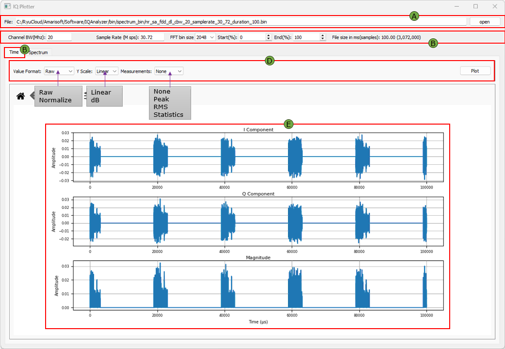
This GUI is organized into a few main areas. Area A is the file selection field. It shows the currently selected IQ file path, and the open button is used to browse and load another IQ file. Area B is the basic configuration area. It shows the channel bandwidth as 20 MHz, the sample rate as 30.72 Msps, the FFT bin size as 2048, and the plotting range from Start 0% to End 100%. It also shows the file size as 100.00 ms, which corresponds to 3,072,000 samples. Area C is the plot mode selection area. The Time tab is selected in this example, so the GUI displays time-domain plots. The Spectrum tab can be selected when you want to inspect the frequency-domain view. Area D is the plot option area. Value Format can be Raw or Normalize, Y Scale can be Linear or dB, and Measurements can be None, Peak, RMS, or Statistics. These options control how the waveform is displayed and what measurement information is added. Area E is the main plotting area. In this Time view, it displays the I component, Q component, and magnitude. The horizontal axis is time in microseconds, and the vertical axis is amplitude. In this example, repeated signal bursts are clearly visible across the 100 ms capture.
(A) File Open
Used to load the binary IQ sample file into the tool for analysis.
- File Path Field displays the full path of the loaded
.binfile. - Open Button opens a file browser to select and load a file.
(B) Common Information
Displays metadata and parameters of the loaded IQ file, including bandwidth, sample rate, and analysis range.
- Channel BW (MHz) sets the channel bandwidth.
- Sample Rate (Msps) defines the sample rate of the data.
- FFT Bin Size specifies the size of FFT applied.
- Start(%) / End(%) determines the portion of the file to be analyzed.
- File Size shows the total duration in milliseconds and the number of samples.
(C) Time Plot Tab
Switches the visualization to time-domain representation of the IQ signal.
(D) Time Plot Options
Provides controls to configure time-domain display format and analysis behavior.
- Value Format toggles between Raw and Normalized values.
- Y Scale switches between Linear and dB scale.
- Measurements enables display of statistical metrics such as Peak, RMS, or none.
- Plot Button applies the selected settings to the time plot.
(E) Time Plots
Displays time-domain graphs for I/Q components and their magnitude.
- I Component shows the real part of the IQ data.
- Q Component shows the imaginary part of the IQ data.
- Magnitude shows the combined amplitude over time.
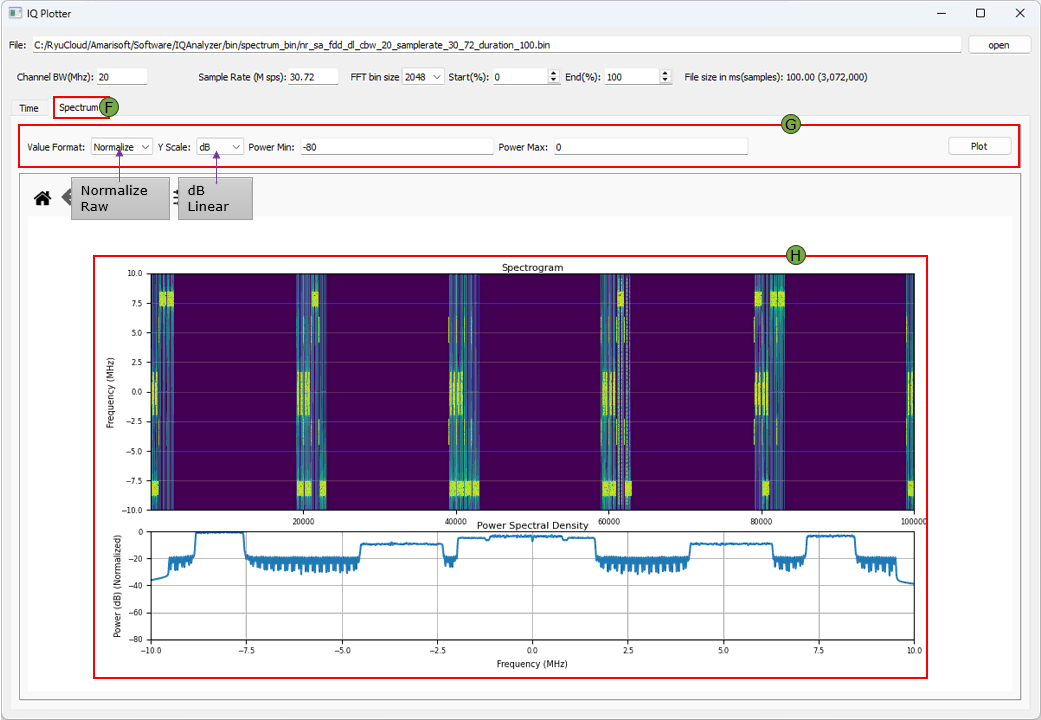
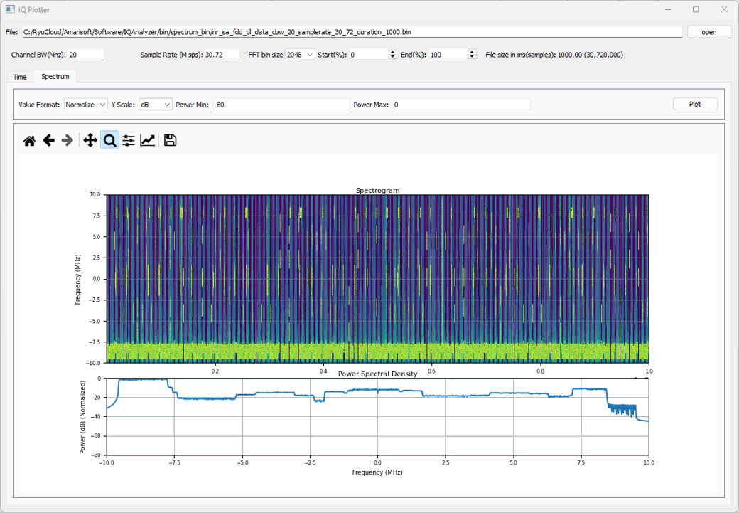
In the view shown below, the Spectrum tab is selected, so the GUI displays the frequency-domain analysis instead of the time-domain waveform. Area F shows the Spectrum tab selection. Area G shows the spectrum plot options. Value Format is set to Normalize, so the spectrum is displayed relative to the normalized reference level. Y Scale is set to dB, so the power level is shown in logarithmic scale. Power Min is set to -80 and Power Max is set to 0, which defines the visible power range of the spectrogram and PSD plot. Area H is the main spectrum display area. The upper plot is the spectrogram. It shows how the signal energy changes over time and frequency. The horizontal axis is time, and the vertical axis is frequency from about -10 MHz to +10 MHz. The bright vertical regions indicate the time positions where signal bursts exist. The lower plot is the power spectral density. It shows the average frequency-domain power shape across the selected data range. This view is useful when you want to check where the signal is located in frequency, whether the occupied bandwidth fits within the expected 20 MHz channel, and whether the burst timing pattern is consistent over the capture.
(F) Spectrum Plot Tab
Switches the visualization to frequency-domain spectrum analysis.
(G) Spectrum Plot Options
Allows configuration of frequency-domain visualization and scaling.
- Value Format sets display as Raw or Normalized.
- Y Scale chooses between Linear and dB.
- Power Min / Max defines the dB range for spectrum visualization.
- Plot Button applies the selected settings to the spectrum plot.
(H) Spectrum Plots
Displays spectral characteristics of the signal over time and frequency.
- Spectrogram shows the frequency content over time using a color heatmap.
- Power Spectral Density (PSD) shows average power per frequency bin.
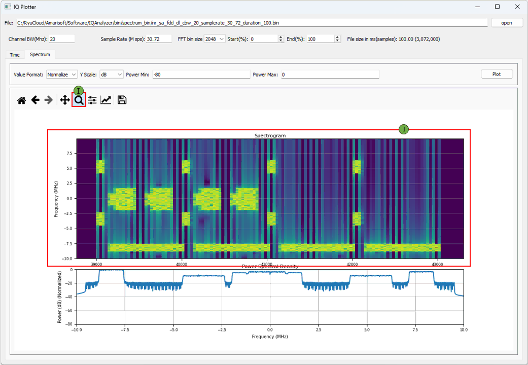
Following view shows how to inspect a smaller region of the spectrogram by using the magnification function. Area I shows the magnification button in the matplotlib toolbar. After selecting this button, you can drag the mouse over the target region in the spectrogram. Area J shows the zoomed spectrogram result. In this example, the display is zoomed into a smaller time range around 39 ms to 43 ms, so the detailed frequency-time structure becomes much easier to see. The bright blocks show where stronger signal energy exists, and the dark vertical gaps show periods with little or no signal energy. This is useful when the full spectrogram is too compressed and you want to check the timing, frequency position, and burst structure of a specific part of the IQ capture.
(I) Zoom
Provides interactive tools to zoom, pan, and reset views for closer inspection of plots. (NOTE : In addition to Zoom, you can use various other toolboxes provided by Python matplotlab)
(J) Zoomed Plot
Shows a magnified view of the spectrogram and PSD, useful for analyzing fine details.
Example 01 : DL signal with SSB, Traffic PDSCH, CSI RS
This is another example carrying more diveserse channels (e.g, Traffic PDSCH, CSI RS etc). You can download the I/Q data here. (
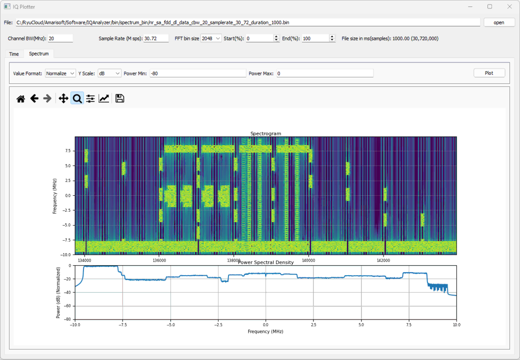
This plot shows the spectrogram for the entire 1 second IQ capture. The file is sampled at 30.72 Msps, so the full file contains 30,720,000 samples. Because this is a large amount of IQ data, the GUI may take some time to read, process, and plot the result. In some environments, you may need to wait several tens of seconds before the spectrogram is displayed. In this example, the Spectrum tab shows the full 0 to 1 second range. The spectrogram shows many vertical activity patterns across time, and the PSD plot at the bottom shows the average frequency-domain power over the whole capture. If you want to reduce the plotting time or inspect only a specific part of the file, you can change Start(%) and End(%) before pressing Plot. For example, plotting only 10% of the file can make the display much faster and easier to inspect.
Following zoomed spectrogram shows a small time segment around the SSB area. Compared with the full 1 second view, this zoomed view makes it much easier to distinguish individual downlink signal components. Around this region, you can see SSB, CORESET 0, PDSCH for SIB, PDSCH for traffic, CSI-RS for TRS, and CSI-RS for CSI report. The strong and wide blocks around the center frequency region correspond to scheduled downlink transmission, while the narrow vertical structures indicate reference signal or control-related activity. The lower PSD plot still shows the average spectrum over the selected range, but the main benefit of this view is the upper spectrogram. It allows you to check when each signal appears, how wide it is in frequency, and how it is positioned relative to the 20 MHz channel bandwidth.