IQ Decode - Python
The purpose of this tutorial is to show how to decode signal from the IQ data. Of course, the purpose is not to provide examples for decoding everything. Decoding every signal and every channel involves the implementation of entire PHY stack which is definitely out of the scope of a tutorial. What I am trying to do in this tutorial is to provide a simple entry point from whichyou can expand and expand.
In this tutorial, I assume that you already have some I/Q data to work with. If you are not familiar with how to capture I/Q, check out following tutorial.
Table of Contents
- IQ Decode - Python
- Introduction
- Summary of the Tutorial
- Disclaimer and Special NOTEs!!!
- Amarisoft as Study and Development tool for PHY
- Test Setup
- Python
- Python Packages
- Python Script - Command Line
- Test 1 : SISO
- Step 1 : Detect LTE PSS and Display (20 Mhz BW)
- Step 2: Detect LTE SSS and Display (20 Mhz BW)
- Step 3: Detect CRS, Estimate Channel Coefficientand Display (20 Mhz BW)
- Step 4: Creation of Channel Coefficient Grid
- Step 5: Equalization
- Test 2: MIMO 2x2
- Step 1: Detect LTE PSS/SSS and Display (20 Mhz BW) for Antenna 0
- Step 2: Construct the Resource Gridfor Antenna 0 and Antenna 1
- Step 3: Construct channel matrix
- Step 4: Equalization
- Step 5: Undo Precoding
- Step 6: Undo Large CDD
- Script - Barebone
- Script - Comments
Introduction
In the field of wireless communications and signal processing, understanding and decoding signals from I/Q (In-phase and Quadrature) data is a foundational skill that enables engineers and researchers to analyze, interpret, and process a wide variety of radio frequency transmissions. I/Q data represents the raw, digitized form of electromagnetic signals captured by software-defined radios (SDRs) or other digital receivers, where the signal is decomposed into its in-phase (I) and quadrature (Q) components. This representation preserves both amplitude and phase information, making it possible to reconstruct the original transmitted waveform and extract meaningful information. The process of decoding signals from I/Q data typically involves several steps, such as filtering, demodulation, symbol decoding, and error correction—each corresponding to layers of the physical (PHY) and data link stack. While the full implementation of a PHY stack for every signal type is a complex endeavor reserved for advanced development, this tutorial provides a practical and accessible entry point for those seeking to begin their journey in signal decoding. By focusing on the fundamentals and essential techniques, learners will gain the foundational knowledge required to interpret I/Q data, paving the way for more advanced exploration and experimentation in the field of digital communications and SDR applications.
-
Context and Background
- I/Q Data Fundamentals: I/Q data consists of two synchronized streams—representing the real (in-phase) and imaginary (quadrature) components of a complex signal—that enable the analysis of both amplitude and phase characteristics of received signals.
- Software-Defined Radio (SDR): SDR platforms facilitate the flexible capture and processing of radio signals by digitizing RF waveforms into I/Q data, which can then be analyzed and decoded in software.
- Role in Signal Processing: Decoding I/Q data is an essential step in extracting information from wireless transmissions, supporting applications in telecommunications, satellite communications, radar, and wireless experimentation.
-
Relevance and Importance of This Tutorial
- Provides a practical introduction to the core steps of decoding signals from I/Q data, serving as a foundation for further study and development in wireless communications.
- Bridges the gap between raw data acquisition and advanced PHY-layer processing, demystifying the initial steps of signal analysis.
- Demonstrates techniques that are widely applicable across a variety of wireless protocols and signal types.
-
Tutorial Objectives and Outcomes
- Understand the structure and format of I/Q data and how it represents RF signals.
- Learn basic methods for visualizing, filtering, and interpreting I/Q samples.
- Apply demodulation and decoding techniques to extract information from I/Q recordings.
- Gain confidence to expand into more advanced signal processing and SDR experimentation.
-
Prerequisite Knowledge and Skills
- Required: Familiarity with digital signal processing concepts, basic understanding of complex numbers, and experience with a programming language (such as Python or MATLAB) used for signal analysis.
- Recommended: Prior exposure to SDR hardware/software and knowledge of radio communications fundamentals.
- Assumption: Learners already have access to I/Q data files. If not, refer to tutorials on capturing and saving I/Q data using tools like sdr_spectrum or remote SDR APIs.
Summary of the Tutorial
This tutorial provides a detailed example of Python-based post-processing of LTE downlink I/Q data, specifically captured using Amarisoft SDR hardware. The tutorial includes two main test cases: one for SISO (Single Input Single Output) and one for MIMO 2x2 (Multiple Input Multiple Output), each demonstrating a sequence of signal processing tasks for LTE physical layer analysis and validation. The focus is on step-by-step methodologies for synchronizing, demodulating, and channel estimating LTE signals using captured I/Q data.
-
Test 1: SISO LTE I/Q Data Processing
-
Step 1: Detect LTE PSS (Primary Synchronization Signal) and Display
- Capture I/Q data using the Amarisoft SDR with specified frequency, bandwidth, and sample rate.
- Detect PSS via cross-correlation with three possible PSS sequences (as per 3GPP) across possible positions in the frequency domain.
- Estimate frequency offset via phase difference analysis of the detected PSS.
- Display results including frequency spectrum, I/Q constellation, expected PSS, and time-domain plots highlighting the detected PSS.
- Extract 14 OFDM symbols around the PSS for further processing.
-
Step 2: Detect LTE SSS (Secondary Synchronization Signal) and Display
- After PSS detection, extract the SSS resource elements from the resource grid at the designated subcarriers.
- Apply frequency offset correction to the SSS symbols.
- Correlate with all possible SSS sequences to identify the correct N_ID_1 and subframe.
- Visualize SSS before and after offset correction, and compare with the generated SSS.
-
Step 3: Detect CRS (Cell-specific Reference Signal), Estimate Channel Coefficient, and Display
- Locate CRS resource elements within the grid using detected PCI and LTE specifications.
- Extract CRS I/Q values from the grid and generate expected CRS per 3GPP for the same positions.
- Estimate the channel by dividing received CRS by expected CRS (h = crs_rx / crs_ex).
- Visualize CRS constellations for each OFDM symbol (symbols 0, 4, 7, 11) and display channel coefficients.
-
Step 4: Creation of Channel Coefficient Grid
- Create a grid the same size as the resource grid and populate it with estimated channel coefficients at CRS positions.
- Interpolate channel coefficients across all resource elements in both time and frequency domains to fill the entire grid.
- Visualize the magnitude and constellation of the interpolated channel coefficient grid.
-
Step 5: Equalization
- Equalize the received signal grid by dividing each resource element by the corresponding channel coefficient from the interpolated grid.
- Visualize the constellation of the resource grid before and after equalization.
-
Step 1: Detect LTE PSS (Primary Synchronization Signal) and Display
-
Test 2: MIMO 2x2 LTE I/Q Data Processing
-
Step 1: Detect LTE PSS/SSS and Display (Antenna 0)
- Load I/Q data for two antennas captured separately for MIMO analysis.
- If necessary, resample the I/Q data to match LTE bandwidth (e.g., from 23.04 MHz to 30.72 MHz for 20 MHz channel).
- Detect PSS and SSS from antenna 0 to acquire synchronization and cell parameters.
-
Step 2: Construct Resource Grids for Both Antennas
- Use synchronization results to extract and construct resource grids for both antennas.
- For each grid, detect SSS, extract CRS, estimate channel coefficients, and interpolate across the grid as in SISO.
- Visualize resource grids and interpolation results for both antennas.
-
Step 3: Construct Channel Matrix (2x2 H Matrix)
- For MIMO, estimate a 2x2 channel matrix at each CRS position using CRS from both antennas and both ports.
- Extract four sets of channel coefficients: h11, h21, h12, and h22, corresponding to each transmit-receive pair.
- Fill and interpolate each channel coefficient grid, then visualize before and after interpolation.
-
Step 4: Equalization (2x2 MIMO)
- For each resource element, form the received vector from both antennas and invert the local H matrix to equalize the received signals.
- Visualize equalized constellations for both antennas.
-
Step 5: Undo Precoding
- Multiply each equalized resource element vector by the inverse of the LTE precoding matrix W to undo transmitter-side precoding.
- Visualize the effect on the constellation.
-
Step 6: Undo Large CDD (Cyclic Delay Diversity)
- First, undo the D matrix (cyclic delay diversity) by multiplying each symbol with the inverse D matrix for that symbol index.
- Then, undo the U matrix by multiplying with its inverse.
- Visualize the final constellation, which should match the expected symbol mapping.
-
Step 1: Detect LTE PSS/SSS and Display (Antenna 0)
Methodology Highlights:
- All signal processing steps follow 3GPP LTE standards for synchronization, resource grid construction, CRS extraction, and channel estimation.
- Python with numpy, scipy, and matplotlib is used for data manipulation, signal processing, and visualization.
- All calculations and corrections (frequency offset, channel estimation, equalization, MIMO matrix inversion, precoding/CDD undoing) are performed explicitly, providing full visibility into each PHY layer procedure.
- The methodology is proof-of-concept and intended for users who wish to validate or develop their own LTE receiver algorithms using real captured I/Q data from Amarisoft SDR hardware.
Disclaimer and Special NOTEs!!!
- The IQ data format should be in Amarisoft I/Q data format (i.e, sequence of 4 Bytes for I and 4 Bytes for Q without any additional file header or meta data)
- The IQ data should be LTE Downlink Signal that carries at least one PSS/SSS (i.e, it should include subframe 0 or subframe 5)
- The sampling rate of the IQ data should be 30.72 Mhz or 23.04Mhz.
- The channel bandwidth should be 20Mhz and the number of RB is 100
Amarisoft as Study and Development tool for PHY
In this tutorial I wanted to propose a new use case of Amarisoft solution which is a study and development tool for physical layer. Probably in most case, the very beginning of PHY layer development would start from purely software based simulation solutions. At this stage, we usually simulate PHY processing (e.g, generation and decode of PHY signal) purely with software.
However, it eventually reach a point where you need to verify our solution with real signal or real hardware. For example, if you are UE PHY reciever developer, you would need real physical gNB transmitter signal for the test. But generating the proper gNB transmitter signal is not easy (especially when you don't have experties on eNB/gNB transmitter chain) and very tedious job to prepare such a signal just for testing. On top of it, the test signal should come from a well verified solution that has proved to be working. If the test signal is not well proved, the entire test result with your own development become unreliable. So in most case we do this (assuming that we want to develope UE side reciever PHY at baseband)
- get a vector signal generator
- get a vector signal analyzer for I/Q capture
- connect the VSG(vector signal generator)and the VSA(vector signal analyzer) and capture IQ data transmitted from VSG
- inject the IQ data into the reciever algorithm that you are developing
Based on my experience, I struggled with most of these steps. Some of the difficulties that I had were :
- VSG and VSA is expensive to get. In order to reduce so additional data preprocessing job and hard work of detailed setting/configuration issues, the generic VSA/VSG function.may not be good enough, you may need to add specific LTE/NR analysis / generation featurewhich push up the cost even further
- Configuration on VSG/VSA is too simple or too complex. Configurations of some VSG/VSA product in the market is too simple. Usually 'too simple' means 'less flexible'. There is not so much of your choice for the output signal patterns that you get. With this, you would not be able to set such a diverse configuration parameters that you see in real gNB/eNB. On the contrary, configurations of some VSG/VSA is too complex. In most case (actually all the VSG/VSA that I have used), those VSA/VSG implements purely low PHY only, no high PHY and MAC. You have to configure all the detailed properties withpurely PHY terms only. This way of configuration is often very tricky.
Why Amarisoft ?
- Cost is much more affordable since the product is purely based on SDR (Software Defined Radio). Except RF front end and DAC/ADC, everything is software
- Embedded IQ capturing tools. The product has embedded vector spectrum analyzer by default. The best environment for your study / development would be to have two Amarisoft product (i.e, Callbox and UEsim), but even with the single box you can transmit a signal and capture IQ simulteneously. In addition, you can capture IQ while the real communication is on going without connecting external equipment (external VSA), splitter/directional coupler/circulator and a lot of cables. Amarisoft callbox/UEsim provide a Remote API to capture both TX and RX IQ.
- Easy configuration with flexibility. Basically Amarisoft product is to provide solution with full stack (i.e, full stack 4G/5G network, full stack 4G/5G UE simulator), so the configuration of the product is designed in such a way to support almost every possible signal patterns that are used in live network and at the same time with easiness that can be understood by most of users.
Test Setup
You can use any kind of test setup that allow you to capture IQ in spectrum Analyzer mode
Python
Following is the version of the python and package that are used for this tutorial. (I tested this on Windows 11 Home Edition). For python, first try with whatever version you are using as long as it is ver 3.x and upgrade it to latest version if it does not work.
- Python version : 3.10.9
Python Packages
For the script in this tutorial, you need to install following packages.
|
pip install numpy pip install matplotlib pip install scipy |
Python Script - Command Line
In this tutorial, I will show you an example of Python script to plot IQ data from a file. This is just an example script intended as POC(Proof of Concept) example. You can revise in any way as you like if this does not suit your purpose.
Test 1 : SISO
By running the script, you would get the test result shown in this section. For the original Python file, click here. For the sample IQ data that you may try with this code, you can download it from here (Unzip the file and change the file name and path in the source code).
Step 1 : Detect LTE PSS and Display (20 Mhz BW)
For this test, I ran a LTE cell with 20Mhz (enb.default.cfg) and capture the TX signal using another sdr card that is not being used for the LTE cell. In my case, I used the sdr card on UEsim, but you can use an SDR card on the callbox which is not being used for the cell. Following is the sdr_spectrum command to capture the IQ data for the this example.
./sdr_spectrum -c 0 -rx_freq 2680e6 -rate 30.72e6 -save-and-exit -duration 0.01 -save_path "/tmp"
If you want to capture the signal with better quality, you may try with the following command
./sdr_spectrum -c 0 -rx_freq 2680e6 -rate 30.72e6 -rx_gain -1 -save-and-exit -duration 0.01 -save_delay 5 -save_path "/tmp"
In this test, the main routine is to detect PSS from the given I/Q data. What is being done in DetectPSS() function can be illustrated as follows.
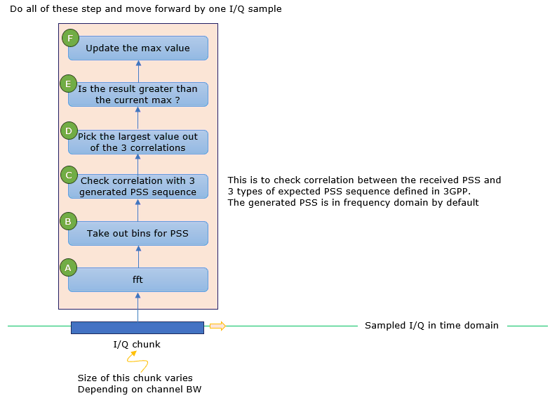
Running the code, you will first get the text output as follows.
|
Detected PSS Sequence (N_ID_2): 0 Maximum correlation: 1.6852206708698385 Maximum correlation for PSS0: 1.6852206708698385 Maximum correlation for PSS1: 1.2416934348611477 Maximum correlation for PSS2: 1.1363440216733818 Position of maximum correlation: 269166 Estimated Frequency Offset: 127120.00185358223 Hz Dimension of resourceGrid = (14, 1199) Detected Subframe : 0 Detected N_ID_2 (PSS) : 0 Detected N_ID_1 (SSS) : 84 Detected PCI: 252 |
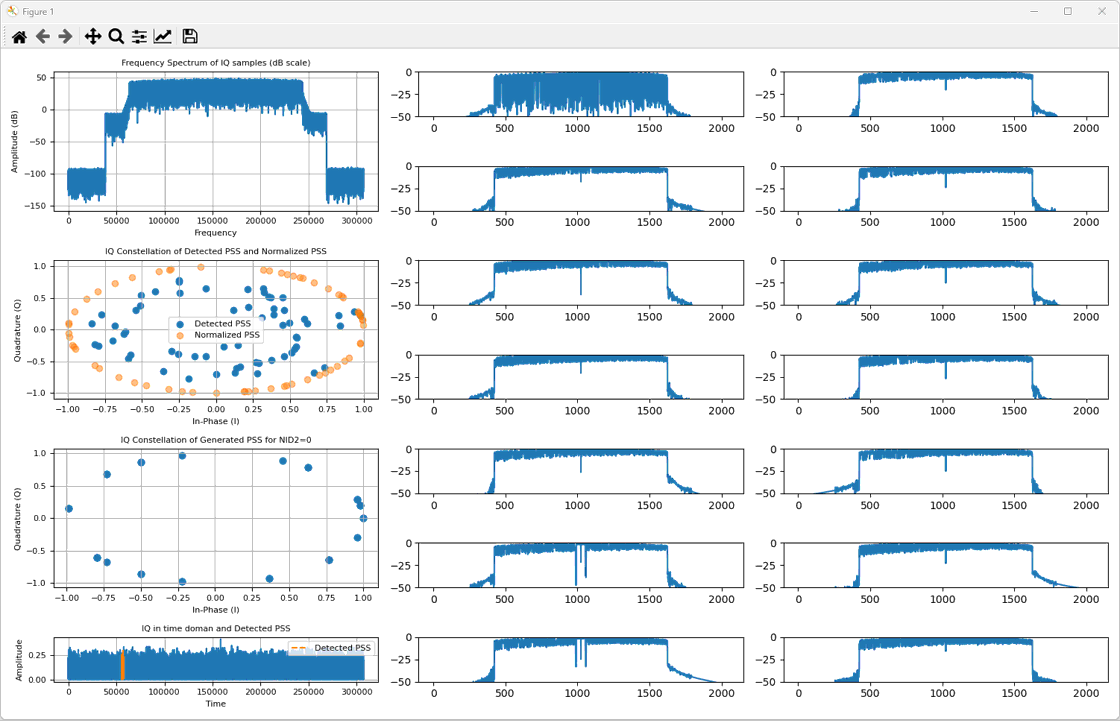
After the detection of PSS, the result is displayed by the function ShowPSS() as follows. This is the output of ShowPSS() function.
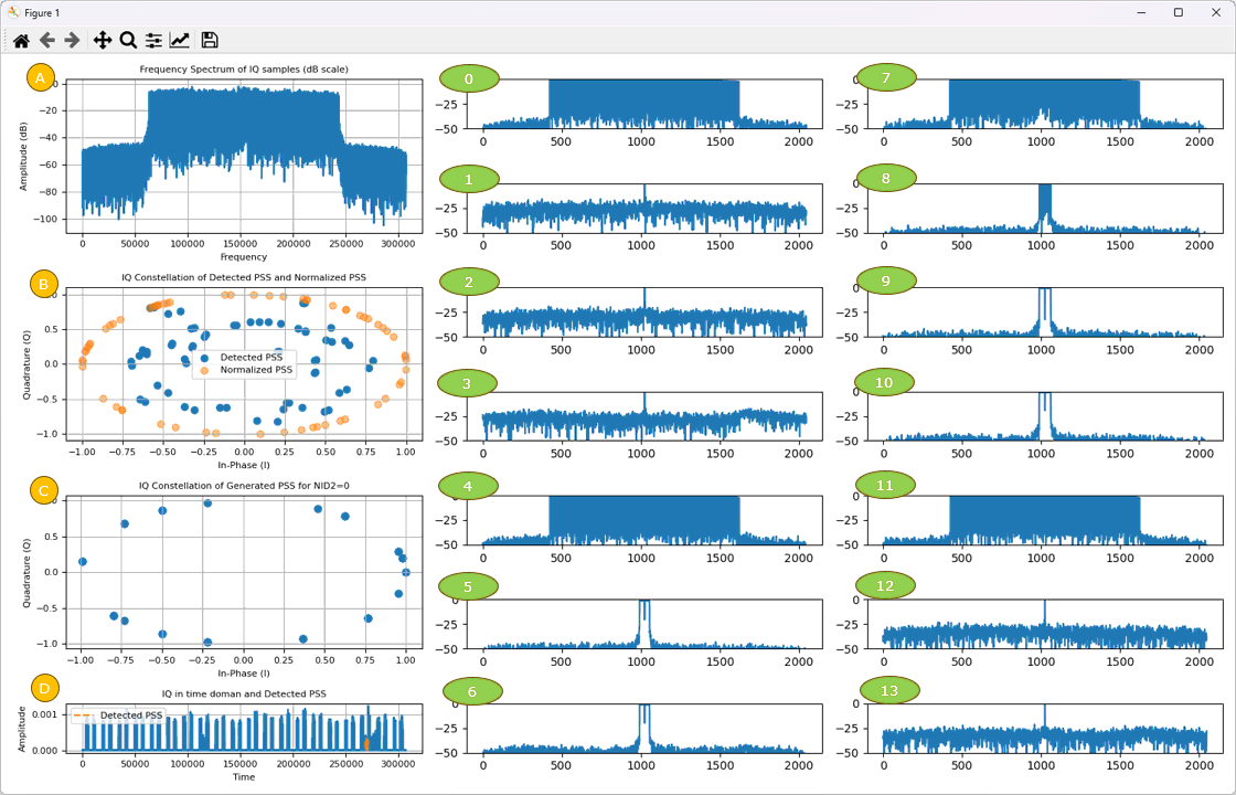
(A) : This is frequency spectrum (plot in frequency) of the entire IQ data given to the program.
(B) : This shows I/Q data in 2D parameteric plot detected from the IQ data. The blue plot shows the I/Q data with magnitue normalized to 1. The plot in orange plot shows the detected PSS sequence with magnitude of all data mapped to 1 reserving angle as it is.
(C) : This shows the expected I/Q data (i.e, The sequence generated by 3GPP spec) corresponding to the detected PSS sequence.
(D) : This is time doman plotof the entire IQ data given to the program. The orange part is the where the detected PSS is located. You can magnify a specific portion of the plot using toolbox at the top of the window.
(0)~(13) : Shows the frequency spectrum for each OFDM symbols within the subframe. (6) is the OFDM symbol where PSS is located.
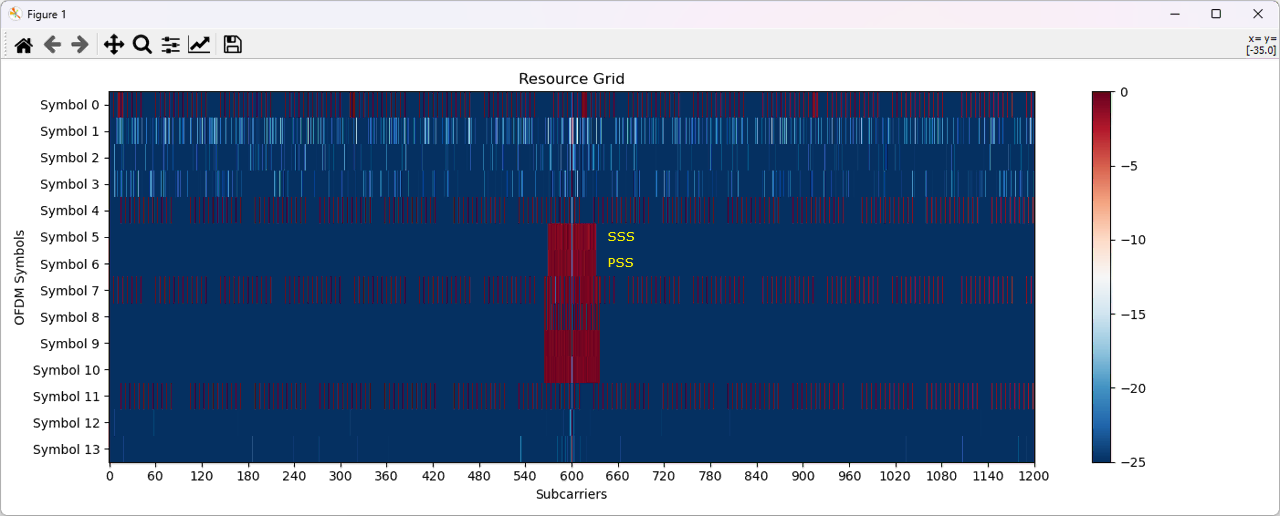
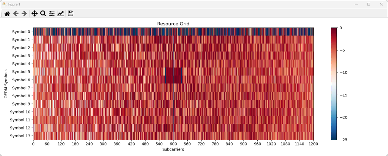
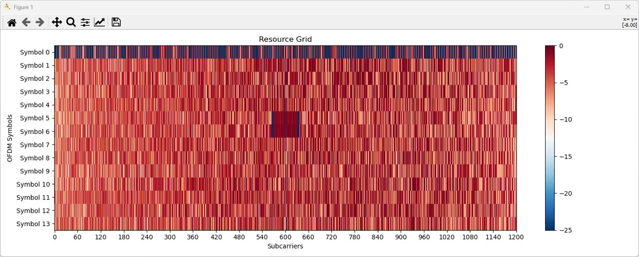
After the PSS detection, we can plot the power of each I/Q data in LTE resource Grid as shown below. This is the output of ShowGrid()
Step 2: Detect LTE SSS and Display (20 Mhz BW)
The overall procedure implemented in this script to detect SSS is illustrated below.
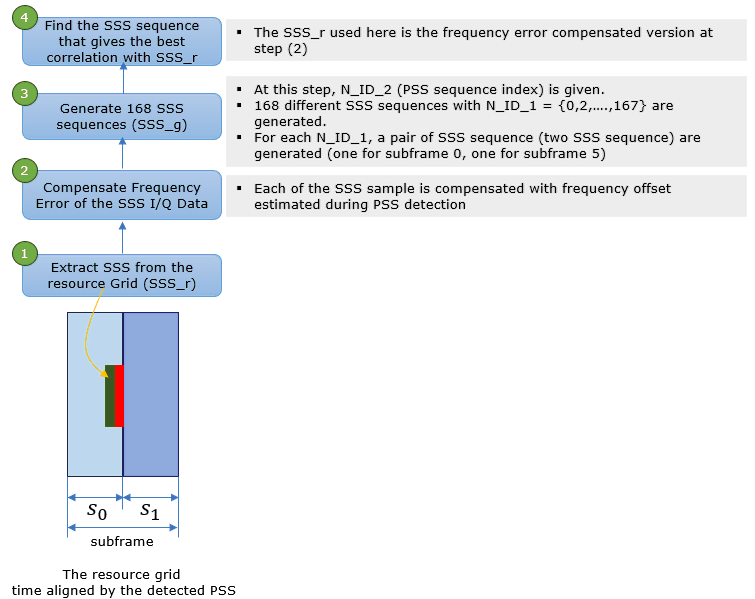
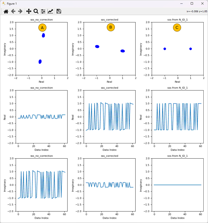
After the PSS detection, it will detect SSS and visualize the detected SSS as below. This is the output of ShowSSS()
Step 3: Detect CRS, Estimate Channel Coefficientand Display (20 Mhz BW)
Once you detected PCI correctly, you can figure out the location of CRS resource elements within the resource grid. If you retrieve the I/Q value in the form of complex number from the CRS resource elements, you will have the list of complex numbers for all the CRS within the subframe.
First run crs_rx, crs_ex, h, crs_k = GetCRSandChannelCoef(resourceGrid, PCI, nRB = 100, method = "generate", subframe=0, debug=False) and run following functions for visualization. Followings are description of arguments and returns.
- resourceGrid : the 2D array that stores all the IQ values for the resourceGrid of one subframe. this is from "resourceGrid = getResourceGrid()" at step 1
- PCI : Physical ID of the cell. This is from "PCI = getPCI(N_ID_1, N_ID_2)" after step 2.
- nRB : The number of RBs within the resourceGrid.
- method : This indicates how to generate the expected crs. "generate" generate the CRS based on 3GPP specification, "testvector" uses a predefined(hardcoded) reference CRS which is produced for PCI 252, nRB100, subframe number 0. I used "testvector" onlyfor debugging purpose.
- subframe : Subframe number within a radio frame
- debug : indicates whether to print out debug print or not
- crs_k : returns a 2D array that stores the resouce elements index of CRS at OFDM symbol 0, 4, 7, 11
- crs_rx : returns a 2D array that stores the resouce elements values retrieved from resourceGrid
- crs_ex : returns a 2D array that stores the resouce elements values generated based on 3GPP specification
- h : returns a 2D array that stores channel coefficient estimated from crs_rx and crs_ex. For SISO with the assumption of low noise channel, it is estimated by h = crs_rx / crs_ex
Followings are constellations and I/Q sequence plot for CRS (Cell Reference Signal) from the detected subframe. (In the constellation, the solid blue indicates the CRS at the lowest frequency and the solid red indcates the CRS at the highest frequency). This is the output of ShowCRS().
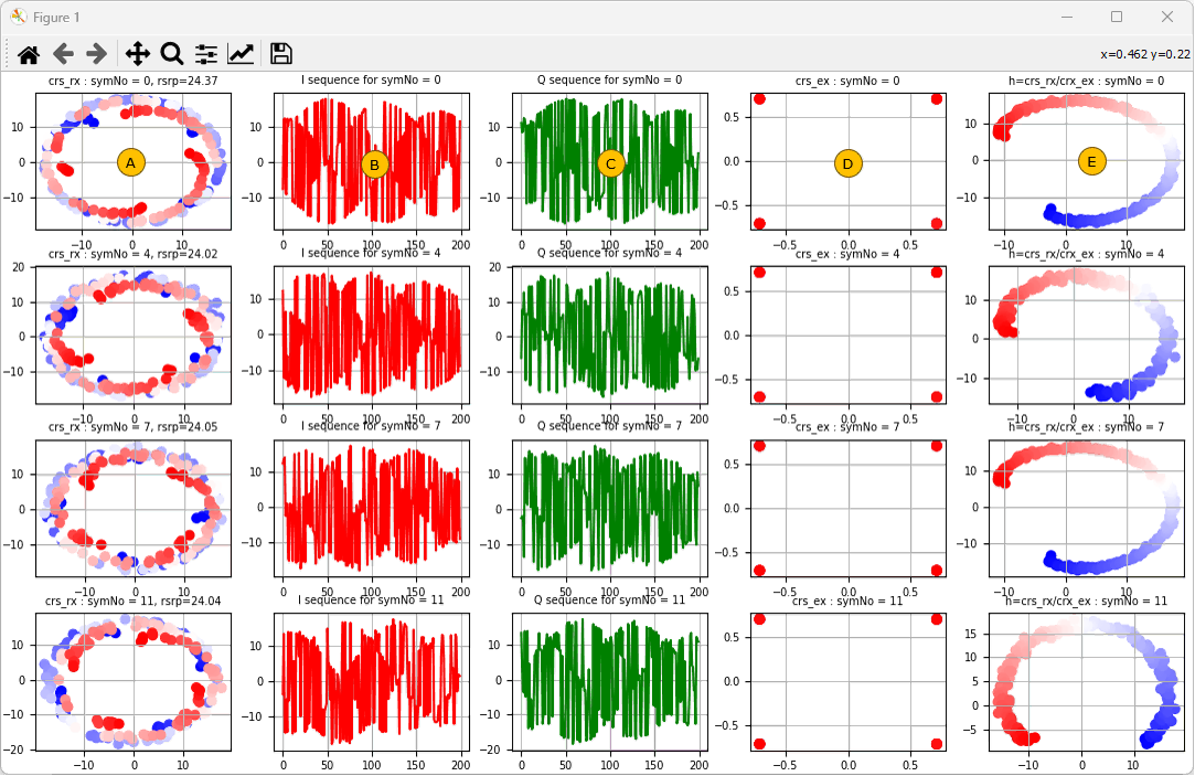
Column (A) : The constellation of CRS retrieved from resourceGrid (these are the received CRS). Rows indicates symbol 0, 4, 7, 11
Column (B), (C): I and Q sequence of the CRS retrieved from resourceGrid. Rows indicates symbol 0, 4, 7, 11
Column(D) : The constellation of CRS generated by 3GPP algorithm. Rows indicates symbol 0, 4, 7, 11
Column(E) : The constellation of channel coefficient estimated from (A) and (D). Rows indicates symbol 0, 4, 7, 11
Step 4: Creation of Channel Coefficient Grid
At this step, I will create a resource grid filled with channel coefficient at each and every resource elements. This is done in a sequence of multiple steps listed below.
First run following functions :
hResourceGrid = cloneArray(resourceGrid, 0.0+1j*0.0) # create a resource grid (hResourceGrid)with the same dimension as "resourceGrid". All the resource elements are initialized with 0.0+1j*0.0
hResourceGrid = setResourceGrid(hResourceGrid, symb=0, k_list=crs_k[0], v_list=h[0]) # fill the channel cofficients stored in h[0] array (channel coefficient for CRS at OFDM symbol 0) atthe OFDM symbol 0 of hResourceGrid
hResourceGrid = setResourceGrid(hResourceGrid, symb=4, k_list=crs_k[1], v_list=h[1]) # fill the channel cofficients stored in h[1] array (channel coefficient for CRS at OFDM symbol 4) atthe OFDM symbol 4 of hResourceGrid
hResourceGrid = setResourceGrid(hResourceGrid, symb=7, k_list=crs_k[2], v_list=h[2]) # fill the channel cofficients stored in h[2] array (channel coefficient for CRS at OFDM symbol 7) atthe OFDM symbol 7of hResourceGrid
hResourceGrid = setResourceGrid(hResourceGrid, symb=11, k_list=crs_k[3], v_list=h[3]) # fill the channel cofficients stored in h[3] array (channel coefficient for CRS at OFDM symbol 11) atthe OFDM symbol 11of hResourceGrid
Then interpolate all non-CRS resource elements based on the h (channel coefficient) values of CRS by running following function. In this function, both frequency domain interpolation and time domain interpolation happens. Frequency domain interpolation is done first and then time-domain interpolation is done.
hResourceGrid_interpolated = interpolateGrid(hResourceGrid, mode = 0, td_method = "interpolate", direction="ccw") and run following functions for visualization
Followings are the descriptions on arguments and returns :
- hResourceGrid : The resource grid on which the interpolation is applied
- mode : specify the mode of the interpolation. 0 : interpolate in both time and frequency, mode 1 for frequency domain only, 2 for time only, 3 for no interpolation
- td_method : specify the method of time domain interpolation. "interpolate" mean to perform interpolation, "copy" mean to copy the coefficient from previoys OFDM symbol.
- direction : specify the direction of angle interpolation between the two complex numbers. "ccw" indicates "counter clock wise". "cw" indicates "clockwise"
- hResourceGrid_interpolated : store the resource grid with all the interpolated coefficient
Then, run following function for visualization.
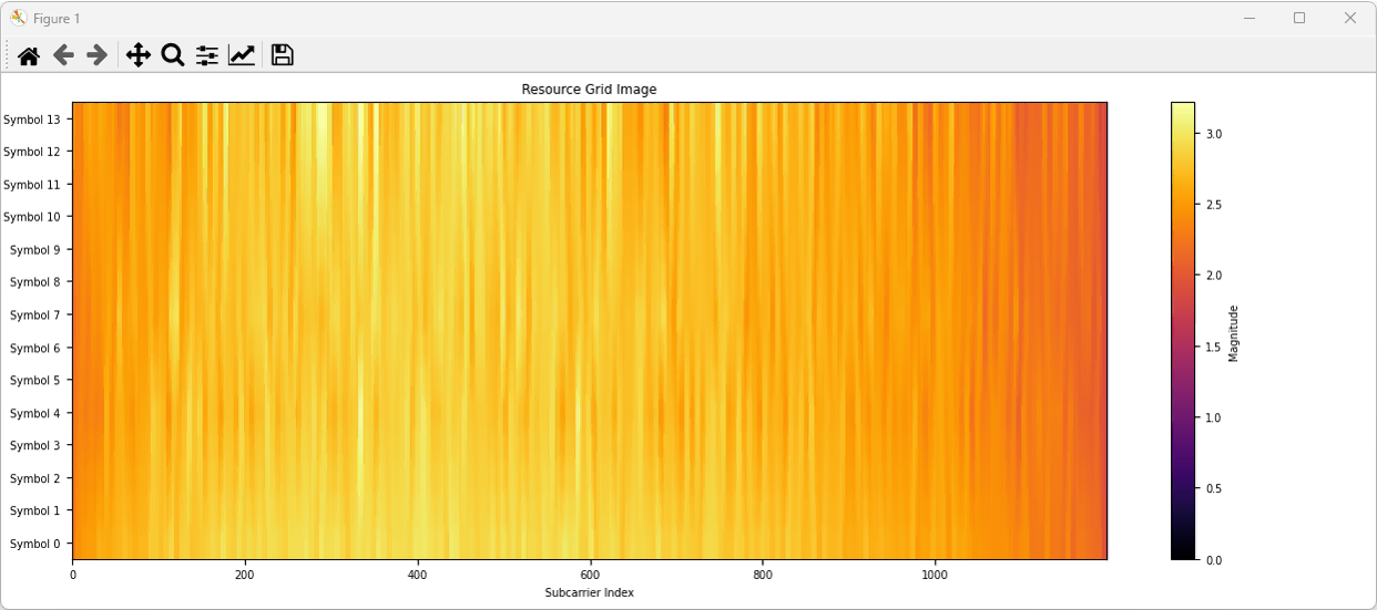
Output ofplotGridImage(hResourceGrid_interpolated). This shows the magnitude of complex numbers (channel coefficient) in every resource elements of the resource grid.
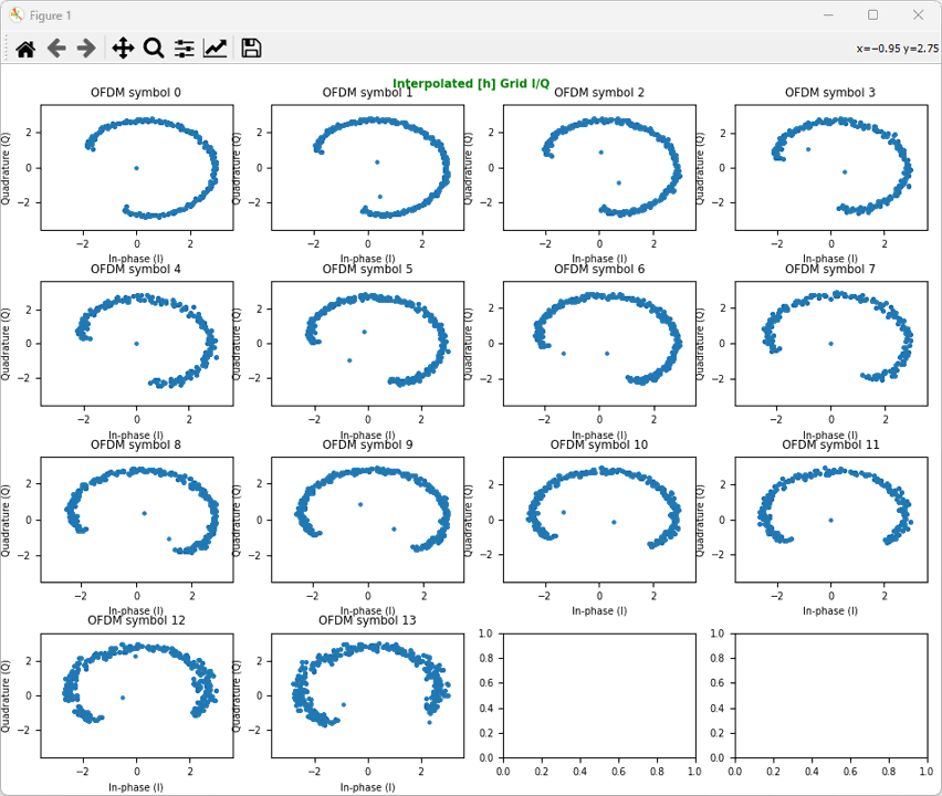
Output of ShowResourceGridIQ(hResourceGrid_interpolated, figTitle="Interpolated [h] Grid I/Q", figTitleColor="green"). This shows the resource elements in every OFDM symbols of the hResourceGrid_interpolated in constellation.
Step 5: Equalization
At this step, I will equalize the received signal using the channel coefficient resource grid (hResourceGrid_interpolated).
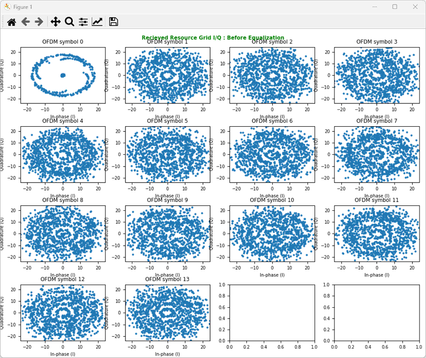
Before equalization, let's plot the constellation of the received signal as it is usingShowResourceGridIQ(resourceGrid, clip = 20, figTitle="Recieved Resource Grid I/Q : Before Equalization", figTitleColor="green")
Then run resourceGrid_corrected = ResourceGridDiv(resourceGrid, hResourceGrid_interpolated) and run following function for visualization. This performs the following operation for each and every resource elements of the resource grids.
resourceGrid_corrected = resourceGrid /hResourceGrid_interpolated
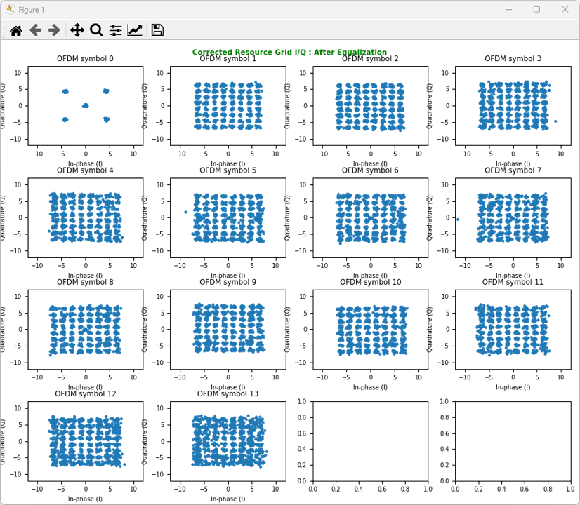
Now, plot the result of the operation using ShowResourceGridIQ(resourceGrid_corrected, clip = 10, figTitle="Corrected Resource Grid I/Q : After Equalization", figTitleColor="green")
Test 2: MIMO 2x2
This test is to show on how to decode 2x2 MIMO IQ data. In terms of fundamental algorithm, the log is same as SISO case. But the complexity of implementation, especially in terms of channel coefficient and equalization. In case of SISO, the channel coefficient is 1x1 (e.g, complex scalar), but in 2x2 MIMO they becomes 2x2 MIMO.
By running the script, you would get the test result shown in this section. For the original Python file, click here. For the sample IQ data that you may try with this code, you can download it from here (Unzip the file and change the file name and path in the source code).
Step 1: Detect LTE PSS/SSS and Display (20 Mhz BW) for Antenna 0
The first step is to detect the PSS and the SSS for Antenna 0. In my implementation, I did this only for Antenna 0 and will use this information to process(i.e, construction of resource grid)Antenna 1 as well.
The script for this step is as follows. Amarisoft Remote API command to capture the 2x2 MIMO captures IQ data and saves into two separate files. So I read each of the files and save it into separate variable iq_samples_p0 and iq_samples_p1.
# read IQ data from a file
iq_samples_p0 = ReadIQ('IQ/lte_20Mhz_rate23.04Mhz_dur_10ms_pci252_traffic_agc_2x2_ota_0.bin')
iq_samples_p1 = ReadIQ('IQ/lte_20Mhz_rate23.04Mhz_dur_10ms_pci252_traffic_agc_2x2_ota_1.bin')
I captured the LTE DL IQ data at UEsim. In UEsim the sample rate for LTE 20Mhz bandwidth is fixed to 23.04Mhz and not allowed to change it to other frequency. Theoretically it is possible to use 23.04 Mhz sampled IQ data for 20Mhz channel bandwidth, but I resampled it to 30.72 which is better fit to 20Mhz channel bandwidth.
# resample the I/Q data sampled at 23.04 to 30.72
iq_samples_p0 = resample_iq(iq_samples_p0, orig_rate=23.04e6, target_rate=30.72e6)
iq_samples_p1 = resample_iq(iq_samples_p1, orig_rate=23.04e6, target_rate=30.72e6)
Now with the resample data, detect PSS and display it only with antenna 0 IQ file.
sample_rate = 30.72e6
fft_bin_size = 2048
NRB = 100
debug_print = False
resultsPSS = DetectPSS(iq_samples_p0,fft_bin_size,sample_rate,debug=debug_print)
ShowPSS(iq_samples_p0, detected_pss_freq_domain, max_correlation_index, ofdm_symbols_p0, pss_start, pss_time_domain, debug = debug_print)
Step 2: Construct the Resource Gridfor Antenna 0 and Antenna 1
With the information obtained from previous step, construct the resource grid for Antenna 0 and Antenna 1 as shown below. These two resource grid is drawn by following two functions.
AnalyzeGrid(resultsPSS, AntPort, ofdm_symbols_p0, NRB, sample_rate, debug_print=debug_print, display = False )
AnalyzeGrid(resultsPSS, AntPort, ofdm_symbols_p1, NRB, sample_rate, debug_print=debug_print, display = False )
Actually this function is an important one and it does many other things in addition to display the resource grid. High level functionality of AnalyzeGrid() function is as follows. (For more details, look into the source code).
1. Extracts various parameters from the `PssInfo` dictionary and other arguments.
2. Calls `getResourceGrid` to get the resource grid from the OFDM symbols.
3. Detects the Secondary Synchronization Signal (SSS) using the `DetectSSS` function.
4. Prints the detected subframe, N_ID_2 (PSS), N_ID_1 (SSS), and the Physical Cell ID (PCI).
5. Displays the resource grid and the SSS if the `display` argument is `True`.
6. Calls `GetCRSandChannelCoef` to calculate the channel coefficient corresponding to each Cell-specific Reference Signals (CRS) and returns the received CRS, channel coefficient, and the list of subcarrier number for CRS.
7. If `display` is `True`, it shows the constellation of received CRS, expected CRS, and the channel coefficient.
8. Creates an empty resource grid and puts the channel coefficient values at the position of each CRS Resource Element (RE).
9. Interpolates the resource grid with the channel coefficients.
10. If `display` is `True`, it plots the interpolated resource grid, I/Q constellation of all 14 OFDM symbols within the specified resource grid, and line graph for each OFDM symbols within the specified resource grid.
11. Corrects/compensates the resource grid with the interpolated channel coefficients.
12. Checks for NaN or Inf values in the corrected resource grid and clips them if found.
13. If `display` is `True`, it plots the I/Q for 14 OFDM symbols of original and corrected resource grid.
14. Returns a dictionary containing the original resource grid, the channel coefficient resource grid, the interpolated channel coefficient resource grid, received CRS, expected CRS, list of subcarrier number for CRS, and the channel coefficient.
Step 3: Construct channel matrix
I have to construct the channel matrix for this 2x2 MIMO case from the two resource grid that I obtained in previous step. In case of SISO, obtaining channel coefficient is relatively simple as shown here and here because the channel coefficient for each resource element is a scalar (complex valued scalar). However, for 2x2 MIMO we need to get an 2x2 matrix for channel coefficient for each resource element. The way the matrix is constructed is illustrated as below.
- h11 = port 0 CRS(Cell Reference Signal) from Antenna 0 resource grid
- h21 = port 0CRS(Cell Reference Signal) from Antenna 1resource grid
- h12 = port 1CRS(Cell Reference Signal) from Antenna 0 resource grid
- h22 = port 1CRS(Cell Reference Signal) from Antenna 1resource grid
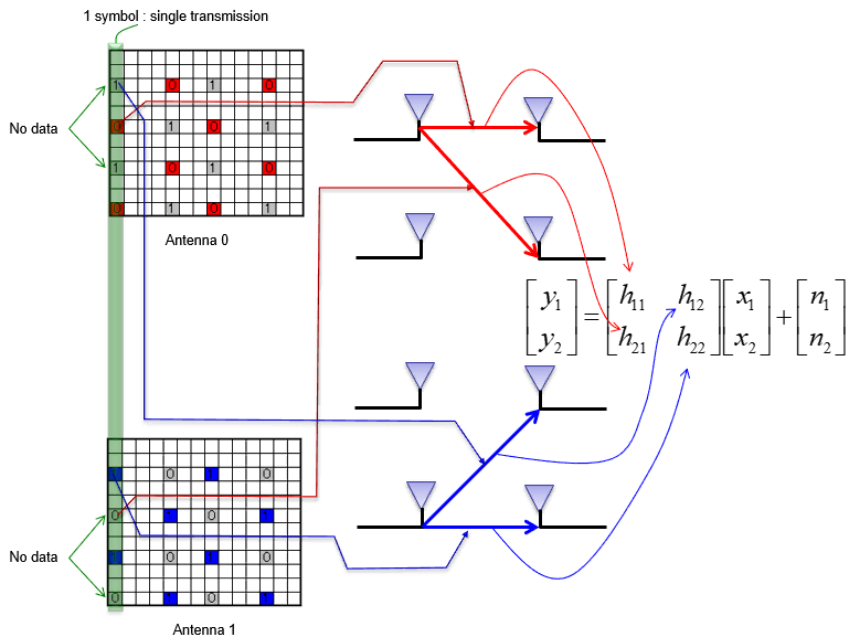
image source : sharetechnote
Once you extracted channel coefficient matrix(H matrix) for every CRS points, we can plot it for visualization. As you see, we get 4 resource grids : h11 grid, h21 grid, h12 grid, h22 grid respectively. The script to do this process is as follows :
The first step is to process the IQ data for Antenn0 and extract CRS for port 0 and port 1, and save them to a separate variables to be easily used for other process
# construct h11 resource grid ************************************************************************************
AntPort = 0
ofdm_symbols_p0 = resultsPSS["ofdm_symbols"]
NRB = 100
sample_rate = 30.72e6
gridInfo_p0 = AnalyzeGrid(resultsPSS, AntPort, ofdm_symbols_p0, NRB, sample_rate, debug_print=debug_print, display = False ) # this function does all the analysis and constructing channel coefficient resource grid
resourceGrid_p0 = gridInfo_p0["resourceGrid"] # this stores the entire resource grid to the variable resourceGrid_p0
h11 = gridInfo_p0["hResourceGrid"] # this extract a resource grid with CRS before interpolation and save the grid to the variable h11
h11_interpolated = gridInfo_p0["hResourceGrid_interpolated"] # this extract a resource grid with CRS afterinterpolation and save the grid to the variable h11_interpolated
crs_rx_p11 = gridInfo_p0["crs_rx"] # this extract the received CRS value to the variable crs_rx_p11. this is 2D array storing the CRS value for the 4 symbols within one subframe
crs_ex_p11 = gridInfo_p0["crs_ex"] # this extract the expected CRS value (CRS value calculated by 3GPP spec) to the variable crs_ex_p11. this is 2D array storing the CRS value for the 4 symbols within one subframe
crs_k_p0 = gridInfo_p0["crs_k"] # this extract the frequency domain RE positions for CRS. this is 2D array storing the CRS value for the 4 symbols within one subframe
h_p11 = gridInfo_p0["h"] #this extract calculated h values. In terms of math, this is just crs_rx_p11/crs_ex_p11. this is 2D array storing the CRS value for the 4 symbols within one subframe
# construct h22 resource grid ************************************************************************************
AntPort = 1
ofdm_symbols_p1 = GetOFDMsymbol(ofdm_symbol_position, iq_samples_p1)
NRB = 100
sample_rate = 30.72e6
gridInfo_p1 = AnalyzeGrid(resultsPSS, AntPort, ofdm_symbols_p1, NRB, sample_rate, debug_print=debug_print, display = False ) # this function does all the analysis and constructing channel coefficient resource grid
resourceGrid_p1 = gridInfo_p1["resourceGrid"] # this stores the entire resource grid to the variable resourceGrid_p1
h22 = gridInfo_p1["hResourceGrid"] # this extract a resource grid with CRS before interpolation and save the grid to the variable h22
h22_interpolated = gridInfo_p1["hResourceGrid_interpolated"]# this extract a resource grid with CRS afterinterpolation and save the grid to the variable h22_interpolated
crs_rx_p22 = gridInfo_p1["crs_rx"] # this extract the received CRS value to the variable crs_rx_p22. this is 2D array storing the CRS value for the 4 symbols within one subframe
crs_ex_p22 = gridInfo_p1["crs_ex"] # this extract the expected CRS value (CRS value calculated by 3GPP spec) to the variable crs_ex_p22. this is 2D array storing the CRS value for the 4 symbols within one subframe
crs_k_p1 = gridInfo_p1["crs_k"] # this extract the frequency domain RE positions for CRS. this is 2D array storing the CRS value for the 4 symbols within one subframe
h_p22 = gridInfo_p1["h"] #this extract calculated h values. In terms of math, this is just crs_rx_p11/crs_ex_p11. this is 2D array storing the CRS value for the 4 symbols within one subframe
Now we have to construct the h resource grid for h21 and h12. As shown above, h11 and h12 were calculated and extracted directedfrom the resource grid for each antenna(resourceGrid_p0 and resourceGrid_p1 respectively), but h21 and h12 can just be extracted from previous two resource grid(resourceGrid_p0 and resourceGrid_p1) without much calculation.
# construct h21 resource grid ************************************************************************************
crs_rx_p21 = []
crs_rx= getREs(resourceGrid_p1, 0, crs_k_p0[0]) # extract the RE value from resourceGrid_p1 at OFDM symbol 0 and frequency domain REs specified by the array crs_k_p0[0]
crs_chest = np.array(crs_rx) / np.array(crs_ex_p11[0]) # calculate the channel coefficient for h21 for all the CRSs at OFDM symbol 0
crs_rx_p21.append(crs_chest) # add the scr_chest to a 2D array crs_rx_p21
crs_rx= getREs(resourceGrid_p1, 4, crs_k_p0[1]) # extract the RE value from resourceGrid_p1 at OFDM symbol 4and frequency domain REs specified by the array crs_k_p0[1]
crs_chest = np.array(crs_rx) / np.array(crs_ex_p11[1])# calculate the channel coefficient for h21 for all the CRSs at OFDM symbol 4
crs_rx_p21.append(crs_chest) # add the scr_chest to a 2D array crs_rx_p21
crs_rx= getREs(resourceGrid_p1, 7, crs_k_p0[2]) # extract the RE value from resourceGrid_p1 at OFDM symbol 7and frequency domain REs specified by the array crs_k_p0[2]
crs_chest = np.array(crs_rx) / np.array(crs_ex_p11[2])# calculate the channel coefficient for h21 for all the CRSs at OFDM symbol 7
crs_rx_p21.append(crs_chest) # add the scr_chest to a 2D array crs_rx_p21
crs_rx= getREs(resourceGrid_p1, 11, crs_k_p0[3]) # extract the RE value from resourceGrid_p1 at OFDM symbol 11and frequency domain REs specified by the array crs_k_p0[3]
crs_chest = np.array(crs_rx) / np.array(crs_ex_p11[3])# calculate the channel coefficient for h21 for all the CRSs at OFDM symbol 11
crs_rx_p21.append(crs_chest) # add the scr_chest to a 2D array crs_rx_p21
h21 = cloneArray(resourceGrid_p1, 0.0+1j*0.0) # create an resource grid, the dimension of which is copied from resourceGrid
# following 4 lines are to populate the blank resoure grid with crs_rx_p21
h21 = setResourceGrid(h21, symb=0, k_list=crs_k_p0[0], v_list=crs_rx_p21[0])
h21 = setResourceGrid(h21, symb=4, k_list=crs_k_p0[1], v_list=crs_rx_p21[1])
h21 = setResourceGrid(h21, symb=7, k_list=crs_k_p0[2], v_list=crs_rx_p21[2])
h21 = setResourceGrid(h21, symb=11, k_list=crs_k_p0[3], v_list=crs_rx_p21[3])
#plotGridImage(h21, "h resource grid : h21")
# interpolate the h21 resource grid
h21_interpolated = interpolateGrid(h21, mode = 0, td_method = "interpolate", direction="ccw")
# construct h12 resource grid ************************************************************************************
crs_rx_p12 = []
crs_rx= getREs(resourceGrid_p0, 0, crs_k_p1[0]) # extract the RE value from resourceGrid_p0 at OFDM symbol 0 and frequency domain REs specified by the array crs_k_p1[0]
crs_chest = np.array(crs_rx) / np.array(crs_ex_p22[0]) # calculate the channel coefficient for h12 for all the CRSs at OFDM symbol 0
crs_rx_p12.append(crs_chest) # add the srs_chest to a 2D array crs_rx_p12
crs_rx= getREs(resourceGrid_p0, 4, crs_k_p1[1]) # extract the RE value from resourceGrid_p0 at OFDM symbol 4and frequency domain REs specified by the array crs_k_p1[1]
crs_chest = np.array(crs_rx) / np.array(crs_ex_p22[1]) # calculate the channel coefficient for h12 for all the CRSs at OFDM symbol 0
crs_rx_p12.append(crs_chest) # add the srs_chest to a 2D array crs_rx_p12
crs_rx= getREs(resourceGrid_p0, 7, crs_k_p1[2]) # extract the RE value from resourceGrid_p0 at OFDM symbol 7and frequency domain REs specified by the array crs_k_p1[2]
crs_chest = np.array(crs_rx) / np.array(crs_ex_p22[2]) # calculate the channel coefficient for h12 for all the CRSs at OFDM symbol 0
crs_rx_p12.append(crs_chest) # add the srs_chest to a 2D array crs_rx_p12
crs_rx= getREs(resourceGrid_p0, 11, crs_k_p1[3]) # extract the RE value from resourceGrid_p0 at OFDM symbol 11and frequency domain REs specified by the array crs_k_p1[3]
crs_chest = np.array(crs_rx) / np.array(crs_ex_p22[3]) # calculate the channel coefficient for h12 for all the CRSs at OFDM symbol 0
crs_rx_p12.append(crs_chest) # add the srs_chest to a 2D array crs_rx_p12
h12 = cloneArray(resourceGrid_p0, 0.0+1j*0.0) # create an resource grid, the dimension of which is copied from resourceGrid
# following 4 lines are to populate the blank resoure grid with crs_rx_p12
h12 = setResourceGrid(h12, symb=0, k_list=crs_k_p1[0], v_list=crs_rx_p12[0])
h12 = setResourceGrid(h12, symb=4, k_list=crs_k_p1[1], v_list=crs_rx_p12[1])
h12 = setResourceGrid(h12, symb=7, k_list=crs_k_p1[2], v_list=crs_rx_p12[2])
h12 = setResourceGrid(h12, symb=11, k_list=crs_k_p1[3], v_list=crs_rx_p12[3])
#plotGridImage(h12, "h resource grid : h12")
# interpolate the h12 resource grid
h12_interpolated = interpolateGrid(h12, mode = 0, td_method = "interpolate", direction="ccw")
Now plot the all 4 channel coefficient before interplation.
gridList = [h11,h21,h12,h22]
titleList = ["h11","h21","h12","h22"]
plotGridTile(gridList, titleList)
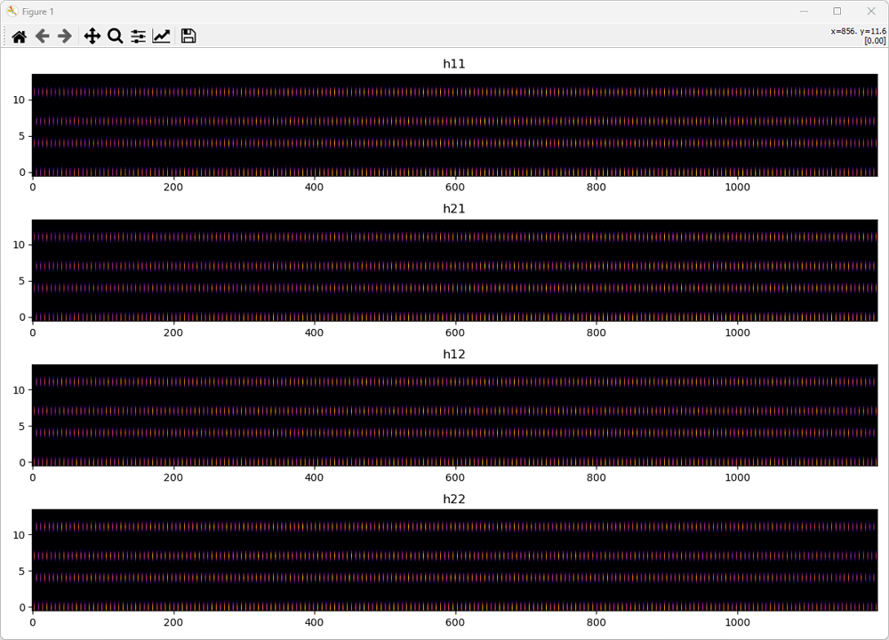
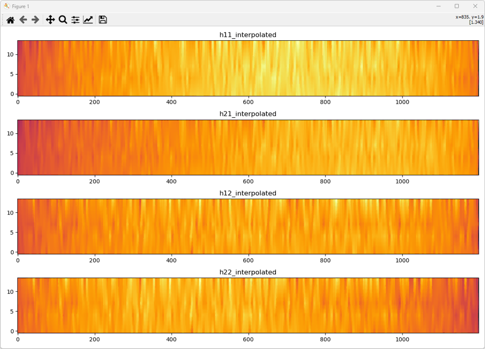
Then perform the interpolation for each resource grid. The algorithm for the interpolation is same as shown for SISO case. I just applied the same algorithm for each resource grid and get the result as shown below.
Now plot the all 4 channel coefficient after interpolation.
gridList = [h11_interpolated,h21_interpolated,h12_interpolated,h22_interpolated]
titleList = ["h11_interpolated","h21_interpolated","h12_interpolated","h22_interpolated"]
plotGridTile(gridList, titleList)
For a little bit different perspective, I plotted the 4 resource grid data into constellation as shown below. The horizontal 14 plots represents the 14 OFDM symbols of the grid and the vertial 4 plots indicates the h11, h21, h12, h22 respectively.
ShowResourceGridIQ_Tile(gridList, TitleList=titleList, clip=5)

Step 4: Equalization
Since we have all the necessary H matrix, we can equalize the received data with the H matrix.
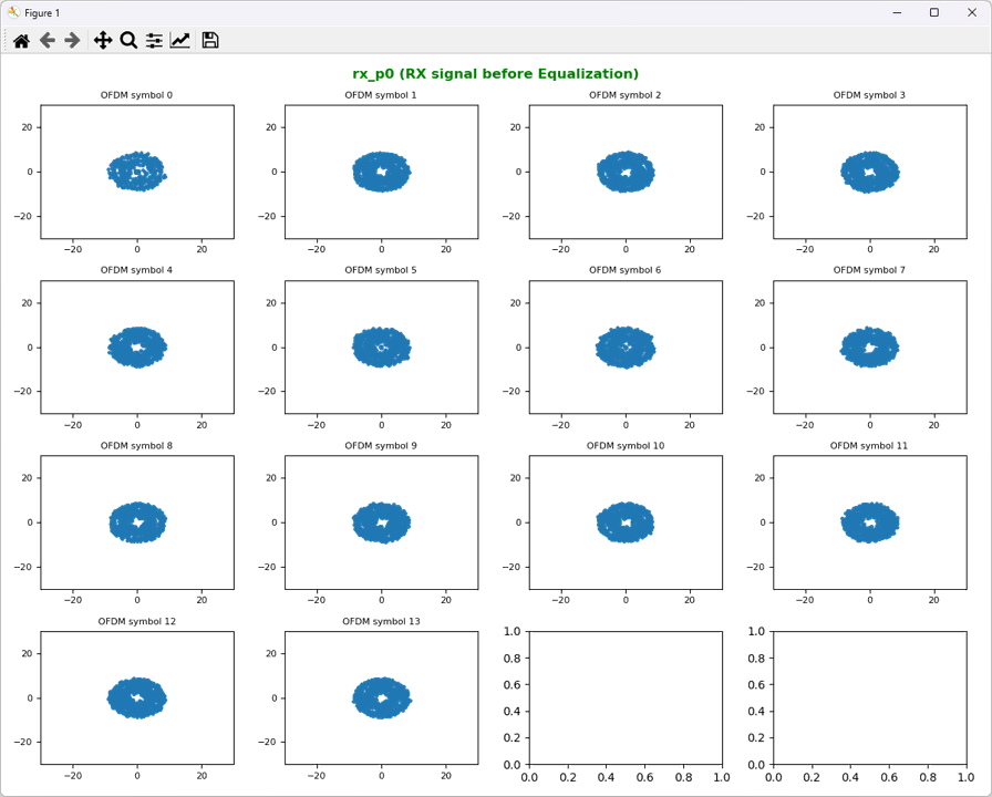
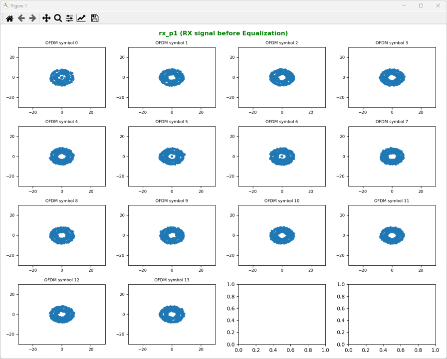
Let's take a look at how the received data look like before equalization. The received data for Antenna 0 (labeled as rx_p0) and Antenna 1(labeled as rx_p1) are look as shown below.
The code to plot these constellation is as follows.
ShowResourceGridIQ(resourceGrid_p0, figTitle="rx_p0 (RX signal before Equalization)", clip = 25, figTitleColor="green")
ShowResourceGridIQ(resourceGrid_p1, figTitle="rx_p1 (RX signal before Equalization)", clip = 25, figTitleColor="green")
Now for the equalization process and processing Precoding / Large CDD, we need a little bit of preparation as below. What we need for this is the interpolated H matrix and W, U, D matrix. So first let's do the preps for this.
Following sixlines are basically changing the name of the variables. This is not mandatary, but I am renaming h11_interpolate to h11 and so on just to use the shorter / simple name.
h11 = h11_interpolated
h21 = h21_interpolated
h12 = h12_interpolated
h22 = h22_interpolated
rx_p0 = resourceGrid_p0
rx_p1 = resourceGrid_p1
Followings are just to make a copy of thd grid structure and assign them to several intermediate variables that will be used in later step. In real implentation, you would not need these kind of resource grids but I am preparing all of these grids to show the plots for all intermediate steps.
rx_p0_eq = resourceGrid_p0.copy()
rx_p1_eq = resourceGrid_p1.copy()
rx_p0_W = resourceGrid_p0.copy()
rx_p1_W = resourceGrid_p1.copy()
rx_p0_D = resourceGrid_p0.copy()
rx_p1_D = resourceGrid_p1.copy()
rx_p0_U = resourceGrid_p0.copy()
rx_p1_U = resourceGrid_p1.copy()
Now let's prepare the matrix for Precoding and Large CDD handling. For 2x2 MIMO, TM3 in LTE, Precoding matrix(W) and large CDD matrix (D and U) are defined as follows by 3GPP. Note that W and U matrix are the matrix with the constant value, but D matrix has the value changing with the position of the data in the given sequence.
W = np.array([
[ 1/np.sqrt(2), 0 ],
[ 0, 1/np.sqrt(2)]
])
def D(i) :
d = np.array([
[ 1, 0 ],
[ 0, np.exp(-1j*(2*np.pi*i/2))]
])
return d
U = np.array([
[ 1/np.sqrt(2), 1/np.sqrt(2) ],
[ 1/np.sqrt(2), np.exp(-1j*(2*np.pi/2))/np.sqrt(2) ]
])
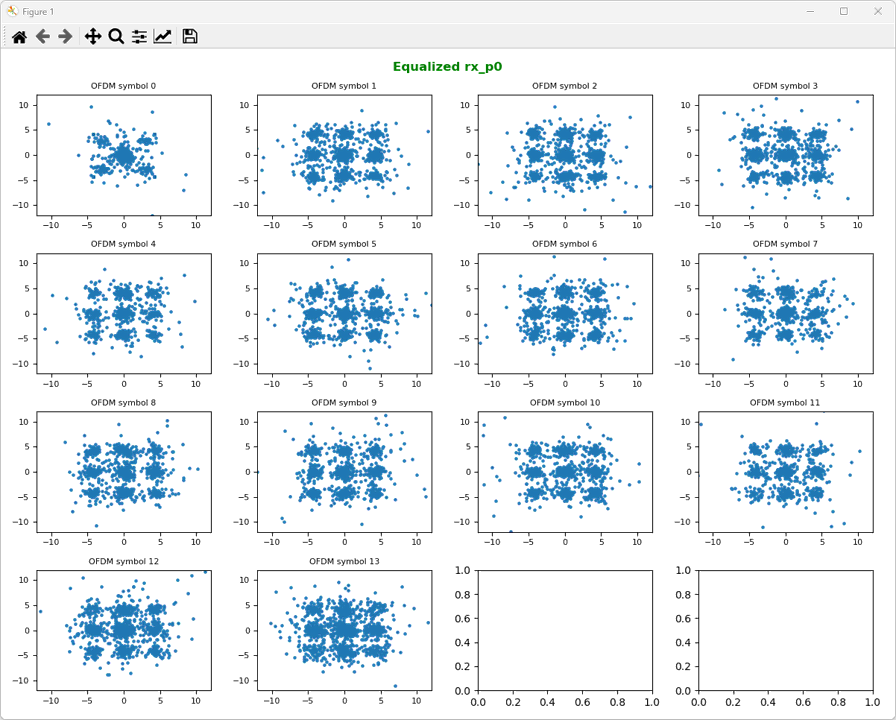
Followings are the result of the equalization for Antenna 0 and Antenna 1. Now you see something looking like a constellation. One thing you may notice would be that this would not look like the constellation that you are expecting. I used the IQ data for 4 QAM Data, but the constellation does not look like QAM except OFDM symbol 0. The reason behind these strange looking constellation is precoding and large CDD which will be processed in following steps.
The code for equalization is as follows. Logic is simple. Multiply each RE data with the inverse of H matrix. Thatis what the two for loops are doing.
for symb in range(len(rx_p0)) :
for k in range(len(rx_p0[1])) :
RX = np.array(
[ [ rx_p0[symb,k] ],
[ rx_p1[symb,k] ]
])
H = np.array([
[ h11[symb,k], h12[symb,k] ],
[ h21[symb,k], h22[symb,k] ]
])
try:
Hinv = np.linalg.inv(H)
except np.linalg.LinAlgError:
# If H is singular, set Hinv to identity matrix
print(f"singular matrix error at ({symb},{k})")
Hinv = np.identity(2)
eq_re = np.dot(Hinv, RX)
rx_p0_eq[symb,k] = eq_re[0]
rx_p1_eq[symb,k] = eq_re[1]
# plot the result into constellation.
ShowResourceGridIQ(rx_p0_eq, figTitle="Equalized rx_p0", clip = 10, figTitleColor="green")
ShowResourceGridIQ(rx_p1_eq, figTitle="Equalized rx_p1", clip = 10, figTitleColor="green")

Step 5: Undo Precoding
In case of LTE MIMO, the transmitted data gets precoded as summarized below. The original data gets applied with large CDD(U and D matrix) first and then gets applied with precoding matrix (W matrix). So at the reciever side (i.e, in decoding process) the process should be done in reverse order. That is, precoding should be undone first and then large CDD should be undone.
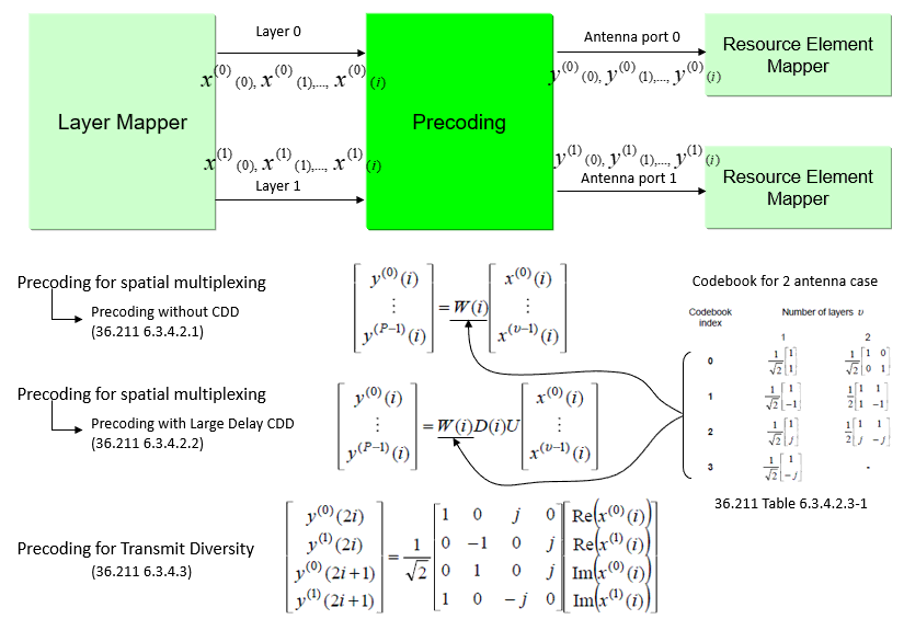
image source : sharetechnote
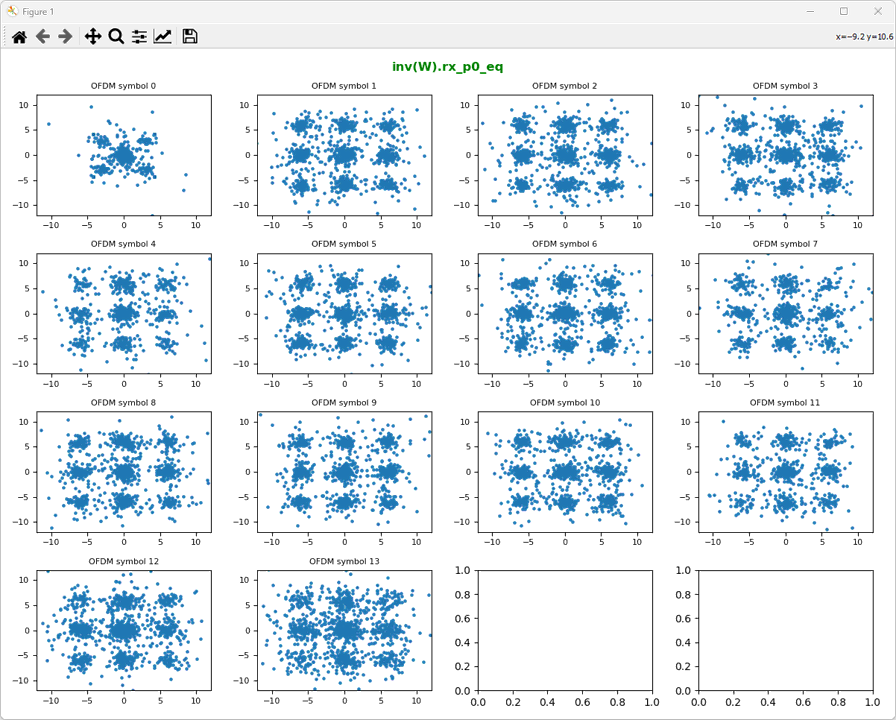
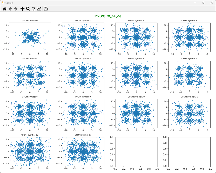
The result of precoding undoing is as follows. Undoing precoding is done simply by multiplying the inverse matrix of precoding matrix W. You would not see much difference even after undoing the precoding just from the constellation. Actually there are a lot of position changes for each symbols (each dots), but the changed position also falls into one of the 9 clusters as before undoing the precoding, so you would not see big difference overall. If you plot all the symbols(dots) in different colors, you may notice some color distributions before and after this process.
In terms of programming logic, this is exactly same as we did in equalization process. Multiply each RE data with the the inverse of precoding matrix(W). Thatis what the two for loops are doing. It is what the two for loops are doing.
for symb in range(len(rx_p0)) :
for k in range(len(rx_p0[1])) :
if symb != 0 :
RX = np.array(
[ [ rx_p0_eq[symb,k] ],
[ rx_p1_eq[symb,k] ]
])
try:
Winv = np.linalg.inv(W)
except np.linalg.LinAlgError:
# If H is singular, set Hinv to identity matrix
print(f"singular matrix error at ({symb},{k})")
Winv = np.identity(2)
eq_re = np.dot(Winv, RX)
rx_p0_W[symb,k] = eq_re[0]
rx_p1_W[symb,k] = eq_re[1]
else:
rx_p0_W[symb,k] = rx_p0_eq[symb,k]
rx_p1_W[symb,k] = rx_p1_eq[symb,k]
ShowResourceGridIQ(rx_p0_W, figTitle="inv(W).rx_p0_eq", clip = 10, figTitleColor="green")
ShowResourceGridIQ(rx_p1_W, figTitle="inv(W).rx_p1_eq", clip = 10, figTitleColor="green")
Step 6: Undo Large CDD
Now we are at the last step which is undoing large CDD. As illustrated below, large CDD is made up of two steps which is multiplication of two matrix U and D. Since U is multiplied and then D is multiplied during large CDD, we have to do this in reverse order in decoding process. That is, undo D matrix first and then undo U matrix.
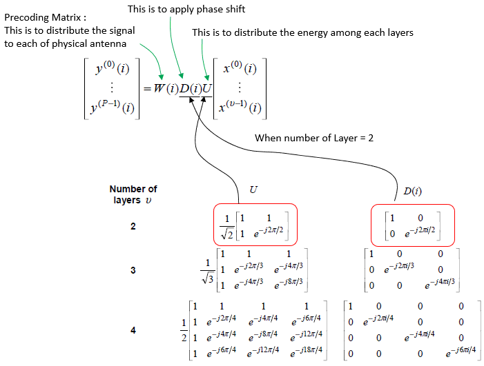
image source : sharetechnote
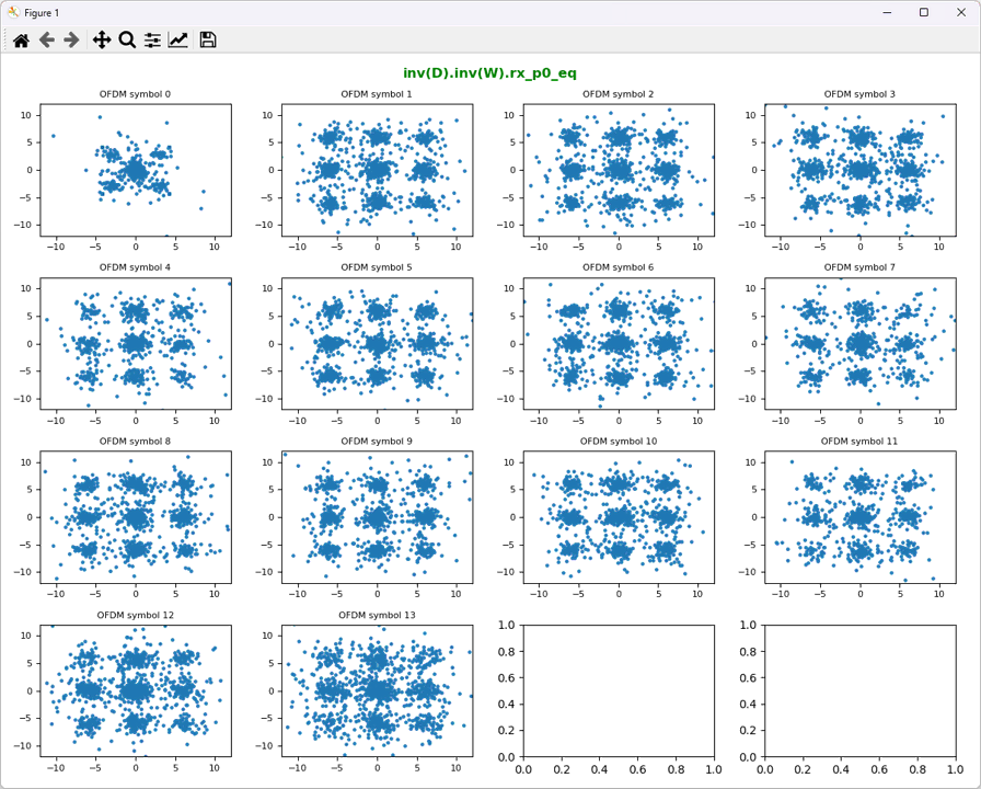
First take a look at the result of undoing D matrix as shown below. Undoing D matrix mean multiplying the inverse matrix of D to data set from previous step.
In terms of programming logic, this is exactly same as we did in previous step. Multiply each RE data with the the inverse of large CDDmatrix(D). Thatis what the two for loops are doing. It is what the two for loops are doing.
for symb in range(len(rx_p0)) :
for k in range(len(rx_p0[1])) :
if symb != 0 :
RX = np.array(
[ [ rx_p0_W[symb,k] ],
[ rx_p1_W[symb,k] ]
])
try:
Dinv = np.linalg.inv(D(k))
except np.linalg.LinAlgError:
# If H is singular, set Hinv to identity matrix
print(f"singular matrix error at ({symb},{k})")
Dinv = np.identity(2)
eq_re = np.dot(Dinv, RX)
rx_p0_D[symb,k] = eq_re[0]
rx_p1_D[symb,k] = eq_re[1]
else:
rx_p0_D[symb,k] = rx_p0_eq[symb,k]
rx_p1_D[symb,k] = rx_p1_eq[symb,k]
ShowResourceGridIQ(rx_p0_D, figTitle="inv(D).inv(W).rx_p0_eq", clip = 10, figTitleColor="green")
ShowResourceGridIQ(rx_p1_D, figTitle="inv(D).inv(W).rx_p1_eq", clip = 10, figTitleColor="green")

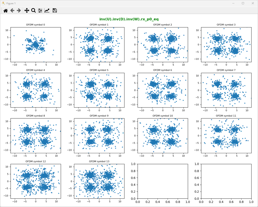
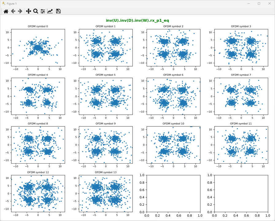
As the last step, let's undo U matrix andtake a look at the result as shown below. Undoing Umatrix mean multiplying the inverse matrix of Uto data set from previous step. Now we get the constellation that matches what we are expecting.
As we did in previous steps,just multiply each RE data with the the inverse of large CDDmatrix(U). Thatis what the two for loops are doing. It is what the two for loops are doing.
for symb in range(len(rx_p0)) :
for k in range(len(rx_p0[1])) :
if symb != 0 :
RX = np.array(
[ [ rx_p0_D[symb,k] ],
[ rx_p1_D[symb,k] ]
])
try:
Uinv = np.linalg.inv(U)
except np.linalg.LinAlgError:
# If H is singular, set Hinv to identity matrix
print(f"singular matrix error at ({symb},{k})")
Uinv = np.identity(2)
eq_re = np.dot(Uinv, RX)
rx_p0_U[symb,k] = eq_re[0]
rx_p1_U[symb,k] = eq_re[1]
else:
rx_p0_U[symb,k] = rx_p0_eq[symb,k]
rx_p1_U[symb,k] = rx_p1_eq[symb,k]
ShowResourceGridIQ(rx_p0_U, figTitle="inv(U).inv(D).inv(W).rx_p0_eq", clip = 10, figTitleColor="green")
ShowResourceGridIQ(rx_p1_U, figTitle="inv(U).inv(D).inv(W).rx_p1_eq", clip = 10, figTitleColor="green")
Script - Barebone
Following is the source script without any comments. I didn't put any comments on purpose for simplicity. For the original Python file, click here. For the sample IQ data that you may try with this code, you can download it from here (Unzip the file and change the file name and path in the source code).
|
import numpy as np import matplotlib.pyplot as plt import struct import matplotlib.gridspec as gridspec from scipy.signal import butter, lfilter
def generate_pss(n_id_2):
u_shift = [25, 29, 34] # Root Zadoff-Chu sequence numbers
d_u = []
for n in range(62): u = u_shift[n_id_2]
if n <= 30: d = np.exp(-1j * np.pi * u * n * (n + 1) / 63) else: d = np.exp(-1j * np.pi * u * (n + 1) * (n + 2) / 63)
d_u.append(d)
return np.array(d_u)
def frequency_offset_estimation(received_pss, expected_pss, sample_rate = 30.72e6):
phase_difference = np.angle(np.dot(received_pss, np.conj(expected_pss))) time_duration_pss = 62 / sample_rate frequency_offset = (phase_difference / (2 * np.pi)) / time_duration_pss
return frequency_offset
def correct_frequency_offset(signal, frequency_offset, sample_rate, debug = False):
if debug : print("[Debug Info] Frequency Offset ==> ",frequency_offset) print("[Debug Info] sample_rate ==> ",sample_rate)
signal = np.array(signal, dtype=np.complex128) time = len(signal) / sample_rate correction = np.exp(-1j * 2 * np.pi * frequency_offset * time) corrected_signal = signal * correction
# just for debugging if debug : original_signal_magnitude = np.abs(signal) corrected_signal_magnitude = np.abs(corrected_signal) # Check if the original signal magnitude and corrected signal magnitude are the same print("comparison of mag : ", np.allclose(original_signal_magnitude, corrected_signal_magnitude)) print("correction : ", correction)
return corrected_signal
def generate_sss(NID1,NID2):
q_prime = np.floor(NID1/30) q = np.floor(((NID1+q_prime*(q_prime+1)/2))/30) m_prime = NID1 + q *(q+1)/2 m0 = m_prime % 31 m1 = (m0 + np.floor(m_prime/31) + 1) % 31
# generate d_even() sequence x_s = np.zeros(31) x_s[:5] = [0, 0, 0, 0, 1] for i in range(26): x_s[i+5] = (x_s[i+2] + x_s[i]) % 2
x_c = np.zeros(31) x_c[:5] = [0, 0, 0, 0, 1] for i in range(26): x_c[i+5] = (x_c[i+3] + x_c[i]) % 2
s_tilda = 1 - 2*x_s c_tilda = 1 - 2*x_c s0_m0_even = np.zeros(31) s1_m1_even = np.zeros(31) for n in range(31): s0_m0_even[n] = s_tilda[int((n+m0)%31)] s1_m1_even[n] = s_tilda[int((n+m1)%31)]
c0_even = np.zeros(31) for n in range(31): c0_even[n] = c_tilda[int((n+NID2)%31)]
d_even_sub0 = s0_m0_even * c0_even d_even_sub5 = s1_m1_even * c0_even
# generate d_odd() sequence x_z = np.zeros(31) x_z[:5] = [0, 0, 0, 0, 1] for i in range(26): x_z[i+5] = (x_z[i+4] + x_z[i+2] + x_z[i+1] + x_z[i]) % 2
z_tilda = 1 - 2*x_z s1_m1_odd = np.zeros(31) s0_m0_odd = np.zeros(31) for n in range(31): s1_m1_odd[n] = s_tilda[int((n+m1)%31)] s0_m0_odd[n] = s_tilda[int((n+m0)%31)]
c1_odd = np.zeros(31) for n in range(31): c1_odd[n] = c_tilda[int((n+NID2+3)%31)]
z1_m0_odd = np.zeros(31) z1_m1_odd = np.zeros(31) for n in range(31): z1_m0_odd[n] = z_tilda[int((n+m0%8)%31)] z1_m1_odd[n] = z_tilda[int((n+m1%8)%31)]
d_odd_sub0 = s1_m1_odd * c1_odd * z1_m0_odd d_odd_sub5 = s0_m0_odd * c1_odd * z1_m1_odd
# calculate d_sub0 d_sub0 = np.zeros(62) d_sub0[::2] = d_even_sub0 d_sub0[1::2] = d_odd_sub0 sss0 = d_sub0
d_sub5 = np.zeros(62) d_sub5[::2] = d_even_sub5 d_sub5[1::2] = d_odd_sub5 sss5 = d_sub5
return sss0, sss5
def cross_correlate(a, b): return np.sum(a * np.conj(b))
def DetectPSS(iq_samples, fft_bin_size=2048):
pss_seqs = [generate_pss(i) for i in range(3)]
max_correlation = 0 max_window_samples = None max_correlation_index = None max_correlation_position = None
max_correlation_pss0 = max_correlation_pss1 = max_correlation_pss2 = 0
for j in range(len(iq_samples) - fft_bin_size): iq_window = iq_samples[j : j + fft_bin_size] frequency_samples = np.fft.fft(iq_window, fft_bin_size) frequency_samples = np.fft.fftshift(frequency_samples)
for k in range(3): window_start = (fft_bin_size - 62) // 2 window_end = window_start + 62 window_samples = frequency_samples[window_start:window_end]
correlation = np.sum(window_samples * np.conj(pss_seqs[k]))
if k == 0 and abs(correlation) > max_correlation_pss0: max_correlation_pss0 = abs(correlation) elif k == 1 and abs(correlation) > max_correlation_pss1: max_correlation_pss1 = abs(correlation) elif k == 2 and abs(correlation) > max_correlation_pss2: max_correlation_pss2 = abs(correlation)
if abs(correlation) > max_correlation: max_correlation = abs(correlation) max_correlation_index = k max_correlation_position = j max_window_samples = window_samples pss_start = j pss_time_domain = np.abs(iq_window)
iq_window = iq_samples[max_correlation_position : max_correlation_position + fft_bin_size] frequency_samples = np.fft.fft(iq_window, fft_bin_size) frequency_samples = np.fft.fftshift(frequency_samples) received_pss = frequency_samples[993:1055] expected_pss = pss_seqs[max_correlation_index] frequency_offset = frequency_offset_estimation(received_pss, expected_pss)
cp_lengths = [160, 144, 144, 144, 144, 144, 144, 160, 144, 144, 144, 144, 144, 144] pss_slot_index = 6
first_symbol_start = (pss_start - cp_lengths[pss_slot_index]) - 5 * (cp_lengths[pss_slot_index]+fft_bin_size) - (cp_lengths[0]+fft_bin_size)
if pss_start >= first_symbol_start + 6 * fft_bin_size and pss_start + 8 * fft_bin_size <= len(iq_samples): ofdm_symbols = [] start_index = first_symbol_start for i in range(14): start_index = start_index + cp_lengths[i] end_index = start_index + fft_bin_size ofdm_symbols.append(iq_samples[start_index : end_index]) start_index = end_index ofdm_symbols = np.array(ofdm_symbols) else: print("Not enough samples to extract 14 OFDM symbols.")
return { 'max_correlation': max_correlation, 'max_correlation_pss0': max_correlation_pss0, 'max_correlation_pss1': max_correlation_pss1, 'max_correlation_pss2': max_correlation_pss2, 'max_correlation_index': max_correlation_index, 'max_correlation_position': max_correlation_position, 'frequency_offset': frequency_offset, 'max_window_samples': max_window_samples, 'ofdm_symbols': ofdm_symbols, 'pss_start' : pss_start, 'pss_time_domain' : pss_time_domain , }
def getREs(ofdm_symbols, symNo, scList):
try: return [ofdm_symbols[symNo][sc] for sc in scList] except IndexError: print("Invalid symbol number or subcarrier index") return []
def ShowPSS(iq_samples, detected_pss_freq_domain, max_correlation_index, ofdm_symbols, pss_start, pss_time_domain, fft_bin_size = 2048):
import matplotlib.pyplot as plt import numpy as np
fig = plt.figure(figsize=(15, 9))
ax1 = plt.subplot2grid((7, 3), (0, 0), rowspan=2, colspan=1) ax3 = plt.subplot2grid((7, 3), (2, 0), rowspan=2, colspan=1) ax4 = plt.subplot2grid((7, 3), (4, 0), rowspan=2, colspan=1) ax5 = plt.subplot2grid((7, 3), (6, 0), rowspan=1, colspan=1)
fft_iq_samples = np.fft.fft(iq_samples) fft_iq_samples = np.fft.fftshift(fft_iq_samples) fft_iq_samples_db = 20 * np.log10(np.abs(fft_iq_samples)) ax1.plot(fft_iq_samples_db) ax1.set_title('Frequency Spectrum of IQ samples (dB scale)', fontsize=8) ax1.grid(True) ax1.set_xlabel('Frequency', fontsize=8) ax1.set_ylabel('Amplitude (dB)', fontsize=8) ax1.tick_params(axis='both', labelsize=8)
fft_detected_pss = np.fft.fft(detected_pss_freq_domain) fft_detected_pss_normalized = fft_detected_pss / np.abs(fft_detected_pss).max()
ax3.scatter(fft_detected_pss_normalized.real, fft_detected_pss_normalized.imag, label='Detected PSS') normalized_data = fft_detected_pss / np.abs(fft_detected_pss) ax3.scatter(normalized_data.real, normalized_data.imag, label='Normalized PSS', alpha=0.5) ax3.legend() ax3.grid(True) ax3.set_title('IQ Constellation of Detected PSS and Normalized PSS', fontsize=8) ax3.set_xlabel('In-Phase (I)', fontsize=8) ax3.set_ylabel('Quadrature (Q)', fontsize=8) ax3.legend(fontsize=8) ax3.tick_params(axis='both', labelsize=8)
generated_pss = generate_pss(max_correlation_index) ax4.scatter(generated_pss.real, generated_pss.imag) ax4.grid(True) ax4.set_title('IQ Constellation of Generated PSS for NID2='+str(max_correlation_index), fontsize=8) ax4.set_xlabel('In-Phase (I)', fontsize=8) ax4.set_ylabel('Quadrature (Q)', fontsize=8) ax4.tick_params(axis='both', labelsize=8)
mag_iq_samples = np.abs(iq_samples) ax5.plot(mag_iq_samples) ax5.plot(range(pss_start, pss_start + len(pss_time_domain)), pss_time_domain, label='Detected PSS', linestyle='--') ax5.grid(True) ax5.set_title('IQ in time doman and Detected PSS', fontsize=8) ax5.set_xlabel('Time', fontsize=8) ax5.set_ylabel('Amplitude', fontsize=8) ax5.legend(fontsize=8) ax5.tick_params(axis='both', labelsize=8)
axs = [plt.subplot2grid((7, 3), (i % 7, i // 7 + 1)) for i in range(14)]
for i in range(14): ax = axs[i] symbol = ofdm_symbols[i] freq_domain_symbol = np.fft.fft(symbol, fft_bin_size) freq_domain_symbol = np.fft.fftshift(freq_domain_symbol) freq_domain_symbol = freq_domain_symbol / np.max(np.abs(freq_domain_symbol)) freq_domain_symbol_db = 20 * np.log10(np.abs(freq_domain_symbol)) ax.plot(freq_domain_symbol_db) ax.set_ylim([-50, 0])
plt.tight_layout() plt.show()
def ShowGrid(ofdm_symbols, nRB = 100, zmin=-25, zmax=0):
frequency_domain_symbols = np.fft.fft(ofdm_symbols, axis=1) frequency_domain_symbols = np.fft.fftshift(frequency_domain_symbols, axes=1)
magnitude = np.abs(frequency_domain_symbols) magnitude = magnitude / np.max(magnitude, axis=1, keepdims=True)
magnitude_db = 20 * np.log10(magnitude + np.finfo(float).eps)
total_subcarriers = frequency_domain_symbols.shape[1]
start_index = (total_subcarriers - nRB * 12) // 2 end_index = start_index + nRB * 12
magnitude_db = magnitude_db[:, start_index:end_index]
fig, ax = plt.subplots(figsize=(14, 5))
cax = ax.imshow(magnitude_db, aspect='auto', cmap='RdBu_r', interpolation='none', vmin=zmin, vmax=zmax)
fig.colorbar(cax)
ax.set_xlabel("Subcarriers") ax.set_ylabel("OFDM Symbols") ax.set_title("Resource Grid")
symbol_labels = ['Symbol {}'.format(i) for i in range(ofdm_symbols.shape[0])] ax.set_yticks(np.arange(ofdm_symbols.shape[0])) ax.set_yticklabels(symbol_labels)
ax.set_xticks(np.arange(0, nRB * 12 + 1, 12*5)) ax.set_xticklabels(np.arange(0, nRB * 12 + 1, 12*5))
plt.tight_layout() plt.show()
def getResourceGrid(ofdm_symbols, nRB = 100): frequency_domain_symbols = np.fft.fft(ofdm_symbols, axis=1) frequency_domain_symbols = np.fft.fftshift(frequency_domain_symbols, axes=1)
total_subcarriers = frequency_domain_symbols.shape[1]
start_index = (total_subcarriers - nRB * 12) // 2 end_index = start_index + nRB * 12
resource_grid = frequency_domain_symbols[:, start_index:end_index]
return resource_grid
def DetectSSS(resourceGrid, N_ID_2, frequency_offset, nRB = 100, samplingRate = 30.72e6, debug = False): if debug : print("[Debug Info] Frequency Offset ==> ",frequency_offset) print("[Debug Info] N_ID_2 ==> ",N_ID_2)
noOfRE = nRB * 12 sss_sc_indices = list(range(noOfRE-noOfRE//2-31, noOfRE-noOfRE//2+31))
sss_no_correction = getREs(resourceGrid, 5, sss_sc_indices) sss = correct_frequency_offset(sss_no_correction, frequency_offset, samplingRate)
max_corr = -np.inf best_N_ID_1 = None for N_ID_1 in range(168): expected_sss0, expected_sss5 = generate_sss(N_ID_1, N_ID_2) corr0 = np.abs(cross_correlate(sss, expected_sss0)) corr5 = np.abs(cross_correlate(sss, expected_sss5)) total_corr = max(corr0, corr5) if debug : print("corr0 = ", corr0, ",corr5 = ", corr5, ", N_ID_1 = ", N_ID_1)
if total_corr > max_corr: max_corr = total_corr best_N_ID_1 = N_ID_1 if debug : print("corr0 = ", corr0, ", corr5 = ", corr5, ", max_corr = ", max_corr, ", N_ID_1 = ", N_ID_1)
if debug : print('Detected SSS (N_ID_1): ', best_N_ID_1)
detected_subframe = 0 if cross_correlate(sss, generate_sss(best_N_ID_1, N_ID_2)[0]) > cross_correlate(sss, generate_sss(best_N_ID_1, N_ID_2)[1]) else 5
return { 'sss_no_correction': sss_no_correction, 'sss_corrected': sss, 'N_ID_1': best_N_ID_1, 'detected_subframe': detected_subframe, }
def getPCI(N_ID_1, N_ID_2) : return 3*N_ID_1 + N_ID_2
def ShowSSS(sss_no_correction, sss_corrected, N_ID_1, N_ID_2,detected_subframe):
sss_generated = np.array(generate_sss(N_ID_1, N_ID_2)) if detected_subframe == 0 : sss_generated = sss_generated[0] else : sss_generated = sss_generated[1]
sss_no_correction = np.array(sss_no_correction, dtype=np.complex128) sss_corrected = np.array(sss_corrected, dtype=np.complex128)
sss_no_correction = sss_no_correction / np.mean(np.abs(sss_no_correction)) sss_corrected = sss_corrected / np.mean(np.abs(sss_corrected))
data_list = [sss_no_correction, sss_corrected, sss_generated ] titles = ['sss_no_correction', 'sss_corrected', 'sss from N_ID_1'] fig, axs = plt.subplots(3, 3, figsize=(9, 9))
for i, data in enumerate(data_list): data = np.array(data, dtype=np.complex128)
axs[0, i].scatter(data.real, data.imag, color='b') axs[0, i].set_title(f'{titles[i]}', fontsize=8) axs[0, i].set_xlabel('Real', fontsize=8) axs[0, i].set_ylabel('Imaginary', fontsize=8) axs[0, i].tick_params(axis='both', which='major', labelsize=8) axs[0, i].set_xlim(-2,2) axs[0, i].set_ylim(-2,2)
axs[1, i].plot(data.real) axs[1, i].set_title(f'{titles[i]}', fontsize=8) axs[1, i].set_xlabel('Data Index', fontsize=8) axs[1, i].set_ylabel('Real', fontsize=8) axs[1, i].tick_params(axis='both', which='major', labelsize=8) axs[1, i].set_ylim(-2,2)
axs[2, i].plot(data.imag) axs[2, i].set_title(f'{titles[i]}', fontsize=8) axs[2, i].set_xlabel('Data Index', fontsize=8) axs[2, i].set_ylabel('Imaginary', fontsize=8) axs[2, i].tick_params(axis='both', which='major', labelsize=8) axs[2, i].set_ylim(-2,2)
plt.tight_layout() plt.show()
def main(): # Load IQ data from binary file with open('IQ/lte_20Mhz_rate30.72Mhz_dur_10ms_pci252.bin', 'rb') as f: # expected PSS Seq = 0 iq_samples = np.fromfile(f, dtype=np.complex64)
resultsPSS = DetectPSS(iq_samples)
print(f'Detected PSS Sequence (N_ID_2): {resultsPSS["max_correlation_index"]}') print(f'Maximum correlation: {resultsPSS["max_correlation"]}') print(f'Maximum correlation for PSS0: {resultsPSS["max_correlation_pss0"]}') print(f'Maximum correlation for PSS1: {resultsPSS["max_correlation_pss1"]}') print(f'Maximum correlation for PSS2: {resultsPSS["max_correlation_pss2"]}') print(f'Position of maximum correlation: {resultsPSS["max_correlation_position"]}') print(f'Estimated Frequency Offset: {resultsPSS["frequency_offset"]} Hz')
max_correlation_index = resultsPSS["max_correlation_index"] pss_start = resultsPSS["pss_start"] pss_time_domain = resultsPSS["pss_time_domain"] ofdm_symbols = resultsPSS["ofdm_symbols"] detected_pss_freq_domain = resultsPSS["max_window_samples"] frequency_offset = resultsPSS["frequency_offset"]
resourceGrid = getResourceGrid(ofdm_symbols, nRB = 100) print("Dimension of resourceGrid = ",resourceGrid.shape)
N_ID_2 = max_correlation_index resultsSSS = DetectSSS(resourceGrid, N_ID_2, frequency_offset, nRB = 100, samplingRate = 30.72e6)
N_ID_1 = resultsSSS["N_ID_1"] sss_no_correction = resultsSSS["sss_no_correction"] sss_corrected = resultsSSS["sss_corrected"] detected_subframe = resultsSSS["detected_subframe"]
print('Detected Subframe : ', detected_subframe)
print('Detected N_ID_2 (PSS) : ', N_ID_2) print('Detected N_ID_1 (SSS) : ', N_ID_1)
PCI = getPCI(N_ID_1, N_ID_2) print('Detected PCI: ', PCI)
ShowPSS(iq_samples, detected_pss_freq_domain, max_correlation_index, ofdm_symbols, pss_start, pss_time_domain) ShowGrid(ofdm_symbols, nRB = 100, zmin = -25, zmax = 0) ShowSSS(sss_no_correction, sss_corrected, N_ID_1, N_ID_2,detected_subframe)
if __name__ == "__main__": main() |
Script - Comments
For the readers who is not familiar with python script and packages that are used in the code. I put the comments for each lines.For the original Python file, click here. For the sample IQ data that you may try with this code, you can download it from here (Unzip the file and change the file name and path in the source code).
|
import numpy as np import matplotlib.pyplot as plt import struct import matplotlib.gridspec as gridspec from scipy.signal import butter, lfilter
def generate_pss(n_id_2):
u_shift = [25, 29, 34]
d_u = []
for n in range(62): u = u_shift[n_id_2]
if n <= 30: d = np.exp(-1j * np.pi * u * n * (n + 1) / 63) else: d = np.exp(-1j * np.pi * u * (n + 1) * (n + 2) / 63)
d_u.append(d)
return np.array(d_u)
def frequency_offset_estimation(received_pss, expected_pss): phase_difference = np.angle(np.dot(received_pss, np.conj(expected_pss))) frequency_offset = phase_difference / (2 * np.pi * 62 / 30.72e6) # Convert phase difference to frequency offset return frequency_offset
def correct_frequency_offset(signal, frequency_offset, sample_rate, debug = False):
if debug : print("[Debug Info] Frequency Offset ==> ",frequency_offset) print("[Debug Info] sample_rate ==> ",sample_rate)
signal = np.array(signal, dtype=np.complex128) time = len(signal) / sample_rate correction = np.exp(-1j * 2 * np.pi * frequency_offset * time) corrected_signal = signal * correction
if debug : original_signal_magnitude = np.abs(signal) corrected_signal_magnitude = np.abs(corrected_signal) print("comparison of mag : ", np.allclose(original_signal_magnitude, corrected_signal_magnitude)) print("correction : ", correction)
return corrected_signal
def generate_sss(NID1,NID2):
q_prime = np.floor(NID1/30) q = np.floor(((NID1+q_prime*(q_prime+1)/2))/30) m_prime = NID1 + q *(q+1)/2 m0 = m_prime % 31 m1 = (m0 + np.floor(m_prime/31) + 1) % 31
x_s = np.zeros(31) x_s[:5] = [0, 0, 0, 0, 1] for i in range(26): x_s[i+5] = (x_s[i+2] + x_s[i]) % 2
x_c = np.zeros(31) x_c[:5] = [0, 0, 0, 0, 1] for i in range(26): x_c[i+5] = (x_c[i+3] + x_c[i]) % 2
s_tilda = 1 - 2*x_s c_tilda = 1 - 2*x_c s0_m0_even = np.zeros(31) s1_m1_even = np.zeros(31) for n in range(31): s0_m0_even[n] = s_tilda[int((n+m0)%31)] s1_m1_even[n] = s_tilda[int((n+m1)%31)]
c0_even = np.zeros(31) for n in range(31): c0_even[n] = c_tilda[int((n+NID2)%31)]
d_even_sub0 = s0_m0_even * c0_even d_even_sub5 = s1_m1_even * c0_even
x_z = np.zeros(31) x_z[:5] = [0, 0, 0, 0, 1] for i in range(26): x_z[i+5] = (x_z[i+4] + x_z[i+2] + x_z[i+1] + x_z[i]) % 2
z_tilda = 1 - 2*x_z s1_m1_odd = np.zeros(31) s0_m0_odd = np.zeros(31) for n in range(31): s1_m1_odd[n] = s_tilda[int((n+m1)%31)] s0_m0_odd[n] = s_tilda[int((n+m0)%31)]
c1_odd = np.zeros(31) for n in range(31): c1_odd[n] = c_tilda[int((n+NID2+3)%31)]
z1_m0_odd = np.zeros(31) z1_m1_odd = np.zeros(31) for n in range(31): z1_m0_odd[n] = z_tilda[int((n+m0%8)%31)] z1_m1_odd[n] = z_tilda[int((n+m1%8)%31)]
d_odd_sub0 = s1_m1_odd * c1_odd * z1_m0_odd d_odd_sub5 = s0_m0_odd * c1_odd * z1_m1_odd
d_sub0 = np.zeros(62) d_sub0[::2] = d_even_sub0 d_sub0[1::2] = d_odd_sub0 sss0 = d_sub0
d_sub5 = np.zeros(62) d_sub5[::2] = d_even_sub5 d_sub5[1::2] = d_odd_sub5 sss5 = d_sub5
return sss0, sss5
def cross_correlate(a, b): return np.sum(a * np.conj(b))
def DetectPSS(iq_samples, fft_bin_size=2048):
pss_seqs = [generate_pss(i) for i in range(3)]
max_correlation = 0 max_window_samples = None max_correlation_index = None max_correlation_position = None
max_correlation_pss0 = max_correlation_pss1 = max_correlation_pss2 = 0
for j in range(len(iq_samples) - fft_bin_size): iq_window = iq_samples[j : j + fft_bin_size] frequency_samples = np.fft.fft(iq_window, fft_bin_size) frequency_samples = np.fft.fftshift(frequency_samples)
for k in range(3): window_start = (fft_bin_size - 62) // 2 window_end = window_start + 62 window_samples = frequency_samples[window_start:window_end]
correlation = np.sum(window_samples * np.conj(pss_seqs[k]))
if k == 0 and abs(correlation) > max_correlation_pss0: max_correlation_pss0 = abs(correlation) elif k == 1 and abs(correlation) > max_correlation_pss1: max_correlation_pss1 = abs(correlation) elif k == 2 and abs(correlation) > max_correlation_pss2: max_correlation_pss2 = abs(correlation)
if abs(correlation) > max_correlation: max_correlation = abs(correlation) max_correlation_index = k max_correlation_position = j max_window_samples = window_samples pss_start = j pss_time_domain = np.abs(iq_window)
iq_window = iq_samples[max_correlation_position : max_correlation_position + fft_bin_size] frequency_samples = np.fft.fft(iq_window, fft_bin_size) frequency_samples = np.fft.fftshift(frequency_samples) received_pss = frequency_samples[993:1055] expected_pss = pss_seqs[max_correlation_index] frequency_offset = frequency_offset_estimation(received_pss, expected_pss)
cp_lengths = [160, 144, 144, 144, 144, 144, 144, 160, 144, 144, 144, 144, 144, 144] pss_slot_index = 6
first_symbol_start = (pss_start - cp_lengths[pss_slot_index]) - 5 * (cp_lengths[pss_slot_index]+fft_bin_size) - (cp_lengths[0]+fft_bin_size)
if pss_start >= first_symbol_start + 6 * fft_bin_size and pss_start + 8 * fft_bin_size <= len(iq_samples): ofdm_symbols = [] start_index = first_symbol_start for i in range(14): start_index = start_index + cp_lengths[i] end_index = start_index + fft_bin_size ofdm_symbols.append(iq_samples[start_index : end_index]) start_index = end_index ofdm_symbols = np.array(ofdm_symbols) else: print("Not enough samples to extract 14 OFDM symbols.")
return { 'max_correlation': max_correlation, 'max_correlation_pss0': max_correlation_pss0, 'max_correlation_pss1': max_correlation_pss1, 'max_correlation_pss2': max_correlation_pss2, 'max_correlation_index': max_correlation_index, 'max_correlation_position': max_correlation_position, 'frequency_offset': frequency_offset, 'max_window_samples': max_window_samples, 'ofdm_symbols': ofdm_symbols, 'pss_start' : pss_start, 'pss_time_domain' : pss_time_domain , }
def getREs(resourceGrid, symNo, scList):
try: return [ofdm_symbols[symNo][sc] for sc in scList] except IndexError: print("Invalid symbol number or subcarrier index") return []
def ShowPSS(iq_samples, detected_pss_freq_domain, max_correlation_index, ofdm_symbols, pss_start, pss_time_domain, fft_bin_size = 2048):
fig = plt.figure(figsize=(15, 9))
ax1 = plt.subplot2grid((7, 3), (0, 0), rowspan=2, colspan=1) ax3 = plt.subplot2grid((7, 3), (2, 0), rowspan=2, colspan=1) ax4 = plt.subplot2grid((7, 3), (4, 0), rowspan=2, colspan=1) ax5 = plt.subplot2grid((7, 3), (6, 0), rowspan=1, colspan=1)
fft_iq_samples = np.fft.fft(iq_samples) fft_iq_samples = np.fft.fftshift(fft_iq_samples) fft_iq_samples_db = 20 * np.log10(np.abs(fft_iq_samples)) ax1.plot(fft_iq_samples_db) ax1.set_title('Frequency Spectrum of IQ samples (dB scale)', fontsize=8) ax1.grid(True) ax1.set_xlabel('Frequency', fontsize=8) ax1.set_ylabel('Amplitude (dB)', fontsize=8) ax1.tick_params(axis='both', labelsize=8)
fft_detected_pss = np.fft.fft(detected_pss_freq_domain) fft_detected_pss_normalized = fft_detected_pss / np.abs(fft_detected_pss).max()
ax3.scatter(fft_detected_pss_normalized.real, fft_detected_pss_normalized.imag, label='Detected PSS') normalized_data = fft_detected_pss / np.abs(fft_detected_pss) ax3.scatter(normalized_data.real, normalized_data.imag, label='Normalized PSS', alpha=0.5) ax3.legend() ax3.grid(True) ax3.set_title('IQ Constellation of Detected PSS and Normalized PSS', fontsize=8) ax3.set_xlabel('In-Phase (I)', fontsize=8) ax3.set_ylabel('Quadrature (Q)', fontsize=8) ax3.legend(fontsize=8) ax3.tick_params(axis='both', labelsize=8)
generated_pss = generate_pss(max_correlation_index) ax4.scatter(generated_pss.real, generated_pss.imag) ax4.grid(True) ax4.set_title('IQ Constellation of Generated PSS for NID2='+str(max_correlation_index), fontsize=8) ax4.set_xlabel('In-Phase (I)', fontsize=8) ax4.set_ylabel('Quadrature (Q)', fontsize=8) ax4.tick_params(axis='both', labelsize=8)
mag_iq_samples = np.abs(iq_samples) ax5.plot(mag_iq_samples) ax5.plot(range(pss_start, pss_start + len(pss_time_domain)), pss_time_domain, label='Detected PSS', linestyle='--') ax5.grid(True) ax5.set_title('IQ in time doman and Detected PSS', fontsize=8) ax5.set_xlabel('Time', fontsize=8) ax5.set_ylabel('Amplitude', fontsize=8) ax5.legend(fontsize=8) ax5.tick_params(axis='both', labelsize=8)
axs = [plt.subplot2grid((7, 3), (i % 7, i // 7 + 1)) for i in range(14)]
for i in range(14): ax = axs[i] symbol = ofdm_symbols[i] freq_domain_symbol = np.fft.fft(symbol, fft_bin_size) freq_domain_symbol = np.fft.fftshift(freq_domain_symbol) freq_domain_symbol = freq_domain_symbol / np.max(np.abs(freq_domain_symbol)) freq_domain_symbol_db = 20 * np.log10(np.abs(freq_domain_symbol)) ax.plot(freq_domain_symbol_db) ax.set_ylim([-50, 0])
plt.tight_layout() plt.show()
def ShowGrid(ofdm_symbols, nRB = 100, zmin=-25, zmax=0):
frequency_domain_symbols = np.fft.fft(ofdm_symbols, axis=1) frequency_domain_symbols = np.fft.fftshift(frequency_domain_symbols, axes=1)
magnitude = np.abs(frequency_domain_symbols) magnitude = magnitude / np.max(magnitude, axis=1, keepdims=True)
magnitude_db = 20 * np.log10(magnitude + np.finfo(float).eps)
total_subcarriers = frequency_domain_symbols.shape[1]
start_index = (total_subcarriers - nRB * 12) // 2 end_index = start_index + nRB * 12
magnitude_db = magnitude_db[:, start_index:end_index]
fig, ax = plt.subplots(figsize=(14, 5))
cax = ax.imshow(magnitude_db, aspect='auto', cmap='RdBu_r', interpolation='none', vmin=zmin, vmax=zmax)
fig.colorbar(cax)
ax.set_xlabel("Subcarriers") ax.set_ylabel("OFDM Symbols") ax.set_title("Resource Grid")
symbol_labels = ['Symbol {}'.format(i) for i in range(ofdm_symbols.shape[0])] ax.set_yticks(np.arange(ofdm_symbols.shape[0])) ax.set_yticklabels(symbol_labels)
ax.set_xticks(np.arange(0, nRB * 12 + 1, 12*5)) ax.set_xticklabels(np.arange(0, nRB * 12 + 1, 12*5))
plt.tight_layout() plt.show()
def getResourceGrid(ofdm_symbols, nRB = 100): frequency_domain_symbols = np.fft.fft(ofdm_symbols, axis=1) frequency_domain_symbols = np.fft.fftshift(frequency_domain_symbols, axes=1)
total_subcarriers = frequency_domain_symbols.shape[1]
start_index = (total_subcarriers - nRB * 12) // 2 end_index = start_index + nRB * 12
resource_grid = frequency_domain_symbols[:, start_index:end_index]
return resource_grid
def DetectSSS(resourceGrid, N_ID_2, frequency_offset, nRB = 100, samplingRate = 30.72e6, debug = False): if debug : print("[Debug Info] Frequency Offset ==> ",frequency_offset) print("[Debug Info] N_ID_2 ==> ",N_ID_2)
noOfRE = nRB * 12 sss_sc_indices = list(range(noOfRE-noOfRE//2-31, noOfRE-noOfRE//2+31))
sss_no_correction = getREs(resourceGrid, 5, sss_sc_indices)
sss = correct_frequency_offset(sss_no_correction, frequency_offset, samplingRate)
max_corr = -np.inf best_N_ID_1 = None for N_ID_1 in range(168): # Generate expected SSS expected_sss0, expected_sss5 = generate_sss(N_ID_1, N_ID_2) # Calculate correlation corr0 = np.abs(cross_correlate(sss, expected_sss0)) corr5 = np.abs(cross_correlate(sss, expected_sss5)) total_corr = max(corr0, corr5) if debug : print("corr0 = ", corr0, ",corr5 = ", corr5, ", N_ID_1 = ", N_ID_1)
if total_corr > max_corr: max_corr = total_corr best_N_ID_1 = N_ID_1 if debug : print("corr0 = ", corr0, ", corr5 = ", corr5, ", max_corr = ", max_corr, ", N_ID_1 = ", N_ID_1)
if debug : print('Detected SSS (N_ID_1): ', best_N_ID_1)
detected_subframe = 0 if cross_correlate(sss, generate_sss(best_N_ID_1, N_ID_2)[0]) > cross_correlate(sss, generate_sss(best_N_ID_1, N_ID_2)[1]) else 5
return { 'sss_no_correction': sss_no_correction, 'sss_corrected': sss, 'N_ID_1': best_N_ID_1, 'detected_subframe': detected_subframe, }
def getPCI(N_ID_1, N_ID_2) : return 3*N_ID_1 + N_ID_2
def ShowSSS(sss_no_correction, sss_corrected, N_ID_1, N_ID_2,detected_subframe):
sss_generated = np.array(generate_sss(N_ID_1, N_ID_2)) if detected_subframe == 0 : sss_generated = sss_generated[0] else : sss_generated = sss_generated[1]
sss_no_correction = np.array(sss_no_correction, dtype=np.complex128) sss_corrected = np.array(sss_corrected, dtype=np.complex128)
sss_no_correction = sss_no_correction / np.mean(np.abs(sss_no_correction)) sss_corrected = sss_corrected / np.mean(np.abs(sss_corrected))
data_list = [sss_no_correction, sss_corrected, sss_generated ] #print("[Debug Info] ==> " , data_list) titles = ['sss_no_correction', 'sss_corrected', 'sss from N_ID_1'] fig, axs = plt.subplots(3, 3, figsize=(9, 9))
for i, data in enumerate(data_list): data = np.array(data, dtype=np.complex128)
axs[0, i].scatter(data.real, data.imag, color='b') axs[0, i].set_title(f'{titles[i]}', fontsize=8) axs[0, i].set_xlabel('Real', fontsize=8) axs[0, i].set_ylabel('Imaginary', fontsize=8) axs[0, i].tick_params(axis='both', which='major', labelsize=8) axs[0, i].set_xlim(-2,2) axs[0, i].set_ylim(-2,2)
axs[1, i].plot(data.real) axs[1, i].set_title(f'{titles[i]}', fontsize=8) axs[1, i].set_xlabel('Data Index', fontsize=8) axs[1, i].set_ylabel('Real', fontsize=8) axs[1, i].tick_params(axis='both', which='major', labelsize=8) axs[1, i].set_ylim(-2,2)
axs[2, i].plot(data.imag) axs[2, i].set_title(f'{titles[i]}', fontsize=8) axs[2, i].set_xlabel('Data Index', fontsize=8) axs[2, i].set_ylabel('Imaginary', fontsize=8) axs[2, i].tick_params(axis='both', which='major', labelsize=8) axs[2, i].set_ylim(-2,2)
plt.tight_layout() plt.show()
def main(): with open('IQ/lte_20Mhz_rate30.72Mhz_dur_10ms_pci252.bin', 'rb') as f: # expected PSS Seq = 0s iq_samples = np.fromfile(f, dtype=np.complex64)
results = DetectPSS(iq_samples)
print(f'Detected PSS Sequence (N_ID_2): {results["max_correlation_index"]}') print(f'Maximum correlation: {results["max_correlation"]}') print(f'Maximum correlation for PSS0: {results["max_correlation_pss0"]}') print(f'Maximum correlation for PSS1: {results["max_correlation_pss1"]}') print(f'Maximum correlation for PSS2: {results["max_correlation_pss2"]}') print(f'Position of maximum correlation: {results["max_correlation_position"]}') print(f'Estimated Frequency Offset: {results["frequency_offset"]} Hz')
max_correlation_index = results["max_correlation_index"] pss_start = results["pss_start"] pss_time_domain = results["pss_time_domain"] ofdm_symbols = results["ofdm_symbols"] detected_pss_freq_domain = results["max_window_samples"]
resourceGrid = getResourceGrid(ofdm_symbols, nRB = 100) print("Dimension of resourceGrid = ",resourceGrid.shape)
# Detect SSS N_ID_2 = max_correlation_index resultsSSS = DetectSSS(resourceGrid, N_ID_2, frequency_offset, nRB = 100, samplingRate = 30.72e6)
N_ID_1 = resultsSSS["N_ID_1"] sss_no_correction = resultsSSS["sss_no_correction"] sss_corrected = resultsSSS["sss_corrected"] detected_subframe = resultsSSS["detected_subframe"]
print('Detected Subframe : ', detected_subframe)
print('Detected N_ID_2 (PSS) : ', N_ID_2) print('Detected N_ID_1 (SSS) : ', N_ID_1)
PCI = getPCI(N_ID_1, N_ID_2) print('Detected PCI: ', PCI)
ShowPSS(iq_samples, detected_pss_freq_domain, max_correlation_index, ofdm_symbols, pss_start, pss_time_domain) ShowGrid(ofdm_symbols, nRB = 100, zmin = -25, zmax = 0) ShowSSS(sss_no_correction, sss_corrected, N_ID_1, N_ID_2,detected_subframe)
if __name__ == "__main__": main()
|